Say I’m trying to characterize a population. One of the best ways to do so is to take the same numeric measurement or measurements from every individual in the population and make a scatterplot of all the data points, to see how they distribute themselves. If we only take one measurement from each individual, then our scatterplot is just a bunch of points on the standard number line. If we take two measurements from each, then our scatterplot is a bunch of points on the standard Cartesian plane. If we take three or more, then our scatterplot is a bunch of points in 3D-space, 4D-space, or higher. The 1-, 2-, 3-, 4-, etc., dimensional space that we plot our points in is the parameter space of our characterization, and each dimension is a parameter.¹ The measurement can belong to the symposition as a whole, or to the symponents, or to the poses between them, or sometimes even abstruse mixes of these or of these and the measuring mechanism. Consequently, a symposition with more symponents will have more potential measurements and thus a higher dimensional parameter space. Ultimately though, the choice of measurements and thus the dimensionality of the parameter space is up to the measurer, but the enumeration of symponents and poses, both at the top levels and down to the substrate, provide a natural parameter space. If I mention a symposition’s parameter space without specifying exactly how it was chosen, then you can assume I mean that natural one that does not include abstruse mixes.

If we add one dimension to our parameter space, we can construct a histogram. A histogram carves up a parameter space into a number of discrete parcels or bins and depicts with the additional dimension how many individuals are plotted in that parcel or bin. A histogram effectively shows the local density of individuals in a subregion of the parameter space. You could call it a “population density landscape,” with peaks in the landscape corresponding to high density. These peaks are called modes. The number of peaks in a histogram depends on both the choice of parameter space and the choice of bins. Consider the population of raindrops that fall during a storm. For reasons related to lightning, raindrops usually carry a small amount of net static electric charge, either positive or negative. If negative, that means there is a tiny fraction of a percent more electrons in the drop than protons; and if positive, a tiny fraction of a percent less. Figure 1 shows a 2-dimensional histogram for raindrops built on a 1-dimensional parameter space with the x-axis being the parameter of charge and the y-axis being a scaled count of raindrops with such charge.

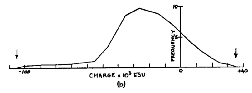
Figure 1. Histogram for the charge of raindrops with a diameter of 1.0 to 1.2 mm. ESU = statcoulombs. http://onlinelibrary.wiley.com/doi/10.1002/qj.49708134705/pdf

The raindrop histogram has one clear mode in the middle. Figure 2 plots stars according to their temperature/color and their luminosity/absolute magnitude. More massive stars tend to be brighter, but even though mass might be a more natural choice of parameter than the brightness, there’s no straightforward way to measure the mass of a star from Earth. The parameter space in Figure 2 is 2-dimensional, and though the additional dimension for the histogram is missing, you can imagine it very easily. The histogram would have at least three modes corresponding to white dwarfs, main sequence starts, and giants, with a possible fourth mode for supergiants if they aren’t just a tail off the distribution of giants.

Figure 2. Hertzsprung-Russell diagram. http://vnatsci.ltu.edu/s_schneider/astro/wbstla2k/mytalk/isoho/hrdiagram.gif

Histograms and parameter spaces take advantage of our natural abilities to visualize and understand physical space. You can flip the conceptual connection and imagine the three ordinary dimensions of space as being a parameter space, with the Dust as datapoints. A histogram constructed from this space as it encompasses the whole Universe would just correspond to the distribution of matter throughout it. In the state immediately after the Big Bang, there was exactly one mode in the distribution, as matter was distributed evenly throughout the hot quark-gluon plasma. Today, matter is quite clumped into many modes corresponding to superclusters, galaxies, planets, rocks, chemicals, etc. The evolving Logos has split the original mode into many modes, each of which sem-links its own many modes contained within. This hierarchy of modes of distribution of matter is, at a rough pass equating position with pose, the partonomy of the Logos, which has been shaped at its top levels by gravity and the bottom levels by the other forces.

But the modes and modes-within-modes of distribution of physical primitives lie strictly within the 3-dimensional “parameter space” of conventional physical space. Any individual symposition is a hierarchy of symponents posed together. If there is a natural parameter space for any symposition, and the dimensions of that space reflect the symposition itself and its symponents and poses, then there is a hierarchy of parameter spaces corresponding to the hierarchy of sympositions where some or all of the dimensions of one space are used in the construction of the dimensions of the space above it. The Dust is constrained to the parameter space of conventional space, but sympositions live in the nearly unbounded parameter space of possibility in the Logos.

Footnotes

1. It’s also called a configuration space and is conceptually similar to feature, phase, and state spaces