Recall that gravity is monovalently attractive. If you had two hydrogen atoms far apart in space, then the parameter space of the symposition of the two would have a dimension corresponding to the distance between them. The distance between them also has a corresponding gravitational potential energy associated with it. Farther distances correspond to more potential energy, and closer distances to less. Energy is conserved, however, so as the hydrogen atoms gravitate towards each other, the gravitational potential energy lost due to their getting closer is converted into kinetic energy, making them move with ever greater velocity as they approach each other. Just like a histogram or population density landscape can be constructed over a parameter space, a potential energy landscape can also be constructed over it as well. The parameter space of the symposition of the two hydrogen atoms has a potential landscape that reaches a minimum or valley when the two atoms are in the same place.

But that analysis is strictly gravitational. Atoms have primitives that also interact according to the other forces. The potential landscape from electromagnetism is more complicated, but suffice it say that it does not go to a minimum when the two hydrogen atoms are in the same place, but rather when they are about 7.4×10^-11 meters apart. The overall potential landscape from the two forces is simply the sum of the two landscapes, at least until even smaller scales where the nuclear forces also become relevant. Since gravity in this context is overwhelmingly weaker than electromagnetism, the distance between the two atoms is almost completely dictated by electromagnetism.

In general, when primitives are attracted to each other by some force, the potential energy of their symposition is highest when they are separate, and vice-versa when they are repulsed, such as with a pair of electrons. Since the Dust was distributed almost homogeneously at the Big Bang, the Universe was born with an enormous reserve of potential energy in its gravitational form. We can repeat the story from Chapter 2 in terms of energy and potential landscapes. As primitives overcame the Jeans limit and collapsed together, the gravitational potential energy was converted into other forms of energy. First, it was converted into the kinetic energy of the primitives racing together. When they reached a sufficient density, the atoms began colliding violently with each other. The collisions often stripped the electrons from their nuclei, converting the kinetic energy of the atoms into the electromagnetic potential energy of the separation of electrons from their nuclei, along with kinetic energy for the dispersal of electrons and nuclei in their own directions.

With the nuclei stripped of their electrons, electron degeneracy pressure no longer walled the nuclei off from each other. The repulsion between nuclei continued, however, with the electromagnetic component of the potential landscape of two nuclei reaching a peak with the nuclei together and fused. The residual strong force component was the opposite, reaching a deep trough with the nuclei fused. The trough was much more narrow than the electromagnetic peak, however, because the residual strong force only operates at much closer distances. Thus the combined potential landscape from the electromagnetic and strong forces had two valleys, one with the nuclei far apart and one with the nuclei fused, separated by a high potential mountain. You can imagine trying to roll a bowling ball over a hill. With a fast enough roll, the ball would overcome the peak and roll into the valley on the other side; with a roll too slow, it would just go up and then come back down on the original side.¹ Nuclei racing together with enough velocity and kinetic energy overcome the barrier of electromagnetic repulsion and enter the valley of residual strong attraction. For nuclei summing to the size of iron, the residual strong valley of fusion is deeper than the unfused valley. When these nuclei fuse, the drop in potential energy from the difference in depth of the valleys is converted to other forms, such as kinetic energy and electromagnetic radiation, or light, which eventually shines into space, illuminating planets like our own.

Ordinary nuclear fusion in stars does not produce elements substantially larger than iron because the depth of the residual strong valley of fusion is overcome by the height of the electromagnetic peak in these elements. The exceptional circumstances for the fusion of elements beyond iron occur during novae and supernovae, stellar explosions, processes which are too complicated to describe in detail here. When elements far beyond iron are created, they are quite often radioactive, with the peaks separating them from their radioactive products being relatively easy to overcome. When they fission or decay and drop back down to elements closer to iron, they release potential energy.

The release of energy from nuclear fission is the primary source of heat within Earth’s core. The gradual cooling of an object can be used to determine how old it is if one has a good estimate for its initial temperature. Lord Kelvin calculated the age of the Earth a century and a half ago using the correct assumption that it originated as molten, but he did not know about nuclear fission, so he underestimated Earth’s 4.5 billion years of age as being near 100 million years. Without radioactivity, Earth’s core would have cooled a long time ago. Once Earth’s core cools, there will no longer be dissipation of energy from it into space. Currently, that dissipation is the primary factor driving the motion of tectonic plates through the convective processes churning in Earth’s mantle. The motion of the plates powers enormous stresses in the solid materials of Earth’s crust. The stresses are carried by distortions in interatomic bonds, such that they are forced out of the comfort of the lowest points of their potential valleys and up the sides of potential mountains. With enough stress, the potential valleys are finally escaped, and the partonomic neighborhoods of the involved atoms can shift quickly in an earthquake. If the earthquake happens under the sea, it can displace massive amounts of water, throwing the sea out of its own potential valley resulting in a tsunami.

Let’s summarize the pathway of potential energy from Big Bang to tsunami. Primordial gravitational potential energy is used to overcome electromagnetic potential barriers to nuclear fusion. Particularly violent events like novae overshoot the lowest potential valley of iron nuclei, storing potential energy in larger radioactive nuclei. The stored nuclear potential energy is released in planet cores through radioactive decay, powering the convection of molten rock and the motion of tectonic plates. The energy from the motion of tectonic plates is stored in stressed interatomic bonds in rock. The electromagnetic potential energy in the stressed bonds is released in earthquakes, where it can differentially raise and lower sea level. The disrupted sea level packs the energy into gravitational potential energy, full circle from the Big Bang, where it dissipates in a series of waves that transfer the energy elsewhere. The overall story is rather simple: primitives want to flow energetically downhill in the landscapes over the parameter spaces of the sympositions they participate in, but they are blocked by many potential barriers. When they do succeed in flowing downhill, they release energy, which in turn interferes with other primitives flowing downhill.

The energy differential between the actual state of a system with its primitives stuck behind potential barriers and the state of the system where all of the primitives have tunneled through their barriers and into their lowest valleys is called exergy. About 5.9 million years ago, the Strait of Gibraltar closed, and the Mediterranean Sea dried up leaving a string of very salty lakes along its floor. This created a large differential in the sea levels of the terrestrial ocean and of the shriveled Mediterranean. You can imagine being an entrepreneur and building a mill on the closed strait, together with some canals to carry oceanic water over a mill-wheel that dumps into the Mediterranean basin. Unfortunately, after about 0.6 million years of hounding investors, your venture didn’t get funded because the strait reopened, triggering the Zanclean Deluge of the Mediterranean basin.² Where there is a differential in the height of the neighboring bodies of water, a mill can be built to extract the exergy of the falling water. If there is no differential, a useful mill cannot be built. But even without the differential, there is still gravitational potential energy because the water on Earth hasn’t collapsed to a black hole.

It is interesting to ask how much of the energy right after the Big Bang was exergy. Apparently quite a bit of it was, and it would be fun if exactly all of it was, but this is an open question in physics. Regardless, we can look into the World and try to find the distribution of exergy. We have already discussed at length the exergy in simple gravitational, chemical, and nuclear systems. A system also has exergy whenever its partonomic neighborhood includes two or more sympositions at different temperatures; the hotter ones have exergy that can be extracted by letting the heat energy flow into the cooler ones. When they all reach the same temperature, no more exergy can be extracted. Aside from these examples, exergy resides in a complicated tangle of volume, pressure, temperature, and other factors, which are studied by the science of thermodynamics. We can see that the Sun harbors an enormous amount of exergy, as does Earth’s core. A simple way to find exergy is to find those sympositions that radiate heat; life forms do, as do electronic devices, automatic machines, and our homes in winter.

When exergy decreases, where does it go? Where did it go when the Atlantic refilled the Mediterranean? The event was probably very loud, so much of the exergy ended up as sound, which is just the coordinated oscillations of interatomic bond lengths of atoms and molecules of air as they are periodically displaced to and fro at the bottom of their potential valleys. These oscillations are also called “phonons.” Incidentally, heat is exactly as the same thing, except it includes all potential valleys, not just the ones of bond length, such as those from bond angles and rotations. Exergy is lost as it diffuses into the maze of partonomic neighborhoods in the Logos, where no symposition can coordinate a regathering of it all. On the surface of the Earth, the potential foothills that it gets lost among are almost always dependent upon electromagnetism, and the last destination for it is as electromagnetic radiation into space.

Finally, it’s worth addressing the relationship between symmetry and energy. Many of you may understand symmetry as being a rough measure of order. When energy is added to a system or partonomic neighborhood, its sympositions jostle about more, and thus one could expect its order to decrease with the addition of the energy. At a first pass, then, it seems that we could expect symmetry to decrease when energy increases. Enter barium titanate, BaTiO₃. Barium titanate is a crystalline compound with interesting electromagnetic properties like photorefractivity and piezoelectricity that melts (or freezes) at 1625 ºC. If you freeze it through the melting point down to room temperature, it passes through a sequence of solid phases³ that have, in order, hexagonal, cubic, tetragonal, orthorhombic, and rhombohedral crystal structure, where each is a variant on the same unit cell symposition of barium, titanium, and oxygen ions. This sequence arranged by decreasing temperature in fact proceeds from more symmetry to less.

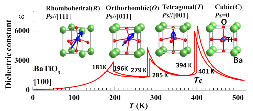
Figure 1. The unit cell of BaTiO₃, at a variety of temperatures, with the dielectric constant plotted. Red spheres are oxygen ions, green barium ions, and blue titanium ions. http://www.intechopen.com/source/html/48777/media/image2.png

A parameter space for the unit cell sympositions for each phase can be constructed whose dimensions measure bond lengths and bond angles between adjacent ions. A small chunk of barium titanate has far more than trillions of ions, so the histogram over the parameter space has similarly many datapoints. Each phase has a different histogram. The hottest phase has the broadest modes, since the individuals are jostling about so much and can’t decide quite where to be, and conversely the coolest phase has the narrowest modes. As the small chunk is cooled, a given mode gets narrower and narrower until a thermodynamic breaking point where it fractures into several pieces. At a high temperature, the titanium ion bounces all around the center of the unit cell, but on average, it is exactly in the middle; at low temperature, the titanium ion picks a direction and shifts off-center, breaking the symmetry with the other ions in the unit cell. Thus the symmetry is broken at the level of interatomic poses, but it is also broken on a higher level: the off-center shift propagates from one unit cell to the next, until it reaches another wave of propagation that decided to shift in another one of the possible directions. If we assume that the small chunk started out at the higher temperature as monocrystalline, that is as a single perfect repeating lattice all throughout, then it can easily end up partitioned into multiple crystal grains, probably separated by twin boundaries.⁴ This partitioning entails the insertion of a level into the partonomy.

We can see that the association between energy and symmetry is the opposite from what one might expect: partonomic neighborhoods with more energy have more symmetry, not less. At the Big Bang, all partonomic neighborhoods were in enormously high energy states, and these correspond to the known homogeneity of the quark-gluon plasma. What happened before the quark-gluon plasma kindles current research into theories of supersymmetry. As the Universe has embarked on lower energy states after the Big Bang,  a cascade of broken symmetries in many partonomic neighborhoods has resulted in a fracturing of populations leading directly to the infilling of partonomic gaps with more levels and the growth of the Logos upon the Dust.

Footnotes

1. A more realistic illustration accounts for the fact that it’s more like two balls participating together in the construction of a hill to divide them.

2. Dramatized by xkcd: http://xkcd.com/1190/

3. In general, a solid of a given compound can have many phases at different temperatures (and pressures), but the compound will have only one liquid phase and only one gaseous phase.

4. http://www.tandfonline.com/doi/abs/10.1080/14786444908561371

The fundamental building block of a partonomy is the relation “part of,” and it links vertically from a lower level to a higher level in a partonomic neighborhood. Sympositions and their symponents do not often belong to the same population because they are rarely particularly similar;¹ thus, a population generally resides on one, given level of a partonomy. Consequently, distillations of populations do have specific vertical localizations in the Logos even though they do not have specific horizontal, i.e. quasi-spatial, localizations like individuals and populations. Similarity, however, is obviously a matter of degree, so a population can be subdivided into subpopulations expressing greater similarity or collected into superpopulations expressing less. Subpopulations and superpopulations can both be distilled, and they can be linked by the horizontal relation “type of” into a hierarchical structure similar to a partonomy. Such a structure is a taxonomy. For instance, with the population of mammals, one can take the subpopulation of primates and the superpopulation of vertebrates. Primates are a type of mammal, and mammals are a type of vertebrate, and these relations extend within the very large and hierarchical Linnaean taxonomy of the “tree of life,” which is both a colorful metaphor and a precise mathematical expression.²

This analysis suggests that taxonomies are always trees. There are two ways in which taxonomies can fail to be trees. Recall the population of raindrops from Figure 1 in the last chapter. Take a raindrop with -30 microstatcoulombs of charge and build a hierarchy of subpopulations that allow for increasingly more variation from it. We can specify the subpopulation of raindrops with -60 to 0 mstatC of charge, and then incorporating that one in a bigger one we can specify the subpopulation of raindrops with -90 to 30 mstatC. We can, however, select a different raindrop with, say, -40 mstatC of charge and build a different hierarchy of subpopulations from it: -70 to -10 mstatC and then -100 to 20 mstatC. These latter sets neither contain nor are able to be contained by their former counterparts. So we have two different and irreconcilable possibilities for the hierarchy of subpopulations of raindrops, neither of which seems ‘better’ in any naïve sense.

The problem, of course, is that I’m forcing hierarchical structure onto the distribution of raindrops when it simply isn’t there. This is true in general for populations with one mode, and we can say that such populations exhibit continuous variation because there is a continuum of possibilities for the relevant parameter with no non-arbitrary location to divide it. Populations that can be divided and for which the divisions can be organized hierarchically exhibit linnaean variation, as the Linnaean taxonomy is the prime example. If you imagine the modes of a population with linnaean variation as being primitives that can be sem-linked, then the partonomy of its histogram is its taxonomy! Once again there is a strong analogy between physical space and parameter spaces, and there is a likeness between the vertical (“part of”) and horizontal (“type of”) orientations in the Logos.

We have only considered a one-dimensional parameter space for the raindrops, that of the charge; we could consider two or more dimensions simultaneously, such as both charge and mass. In that more general case, the raindrops could be said to exhibit multivariate continuous variation, contrasting with the univariate continuous variation over a one-dimensional parameter space. It’s possible that the values of the data points in two or more dimensions of a parameter space are correlated with each other. Raindrops with a greater charge may generally have more mass, but perhaps not in a perfectly predictable way. Thus charge and mass could be correlated in raindrops, but without being interchangeable measures. This correlation would depopulate certain areas of the histogram, but without changing the number of modes. This can be called interdependent multivariate continuous variation, in contrast with independent multivariate continuous variation when there is no correlation. By necessity, all independent and interdependent variation is multivariate, because you need at least two dimensions to have a correlation, so the “multivariate” can be dropped, e.g. as just independent or interdependent continuous variation.

Figure 1. Independent and interdependent continuous variation. On the right, the NW and SE parts of the distribution are slightly underpopulated, and the NE and SW parts of the distribution are slightly overpopulated, making the two parameters correlated. http://www.mdpi.com/applsci/applsci-03-00107/article_deploy/html/images/applsci-03-00107-g001-1024.png

Linnaean variation is a special case of discrete variation, which pertains to those populations that have more than one mode. Every population exhibits exactly one of continuous or discrete variation, given some parameter space like the natural one, since the number of modes is either one or more than one.³ In discrete variation that is not linnaean, the modes cannot be sem-linked together to create a single hierarchical tree. For instance, imagine a population of pea plants that can either be short or tall, depending on some gene with two forms or “alleles,” and can either have constricted or full pods, depending on some other gene with two alleles. Then the individuals have four ways for combining the two characteristics: they can be short with constricted pods, short with full pods, tall with constricted pods, or tall with full pods. The individuals can be plotted in a two-dimensional parameter space of plant height and pod volume. Within this parameter space there will be four modes, each having some small amount of spread. This would be an example of multivariate discrete variation.

The question then arises as to which two pairs of modes should be sem-linked first. Should we have {{{tall and full}_d, {tall and constricted}_d}_d, {{short and full}_d, {short and constricted}_d}_d}_d or {{{tall and full}_d, {short and full}_d}_d, {{tall and constricted}_d, {short and constricted}_d}_d}_d? Neither of these is more forthcoming than the other unless one of height or pod shape is artificially considered primary and the other secondary. Consequently, the taxonomy of the population is not a hierarchical tree, but it is instead a combinatorial crossing between all the possibilities of each allelic modularity. This is basically the same concept as the cartesian product in set theory, so I call such variation cartesian variation. Cartesian variation can be either independent or interdependent, for instance if a pea plant being tall makes it more likely or less likely to have full pods, rather than being neutral.

In sum, there is continuous variation for distributions with one mode and discrete variation for distributions with more than one mode. Discrete variation is perfected in either linnaean or cartesian variation, which are mutually exclusive. Moreover, all of these varieties of variation can be fit into a single framework. Let’s take another detour through math to demonstrate. Pascal’s triangle is a very straightforward mathematical object that is constructed as follows: take a blank sheet of paper and write a “1” in the top center. This will be the first line. Now put zeros on both sides of the one: “0 1 0.” Now for every adjacent pair of numbers on the top line, write their sum in between them on the second line. The first pair, “0 1,” adds to 1, and the second pair, “1 0,” also adds to 1: so the second line is “1 1.” Once again put zeros on both sides of the second line, “0 1 1 0,” and construct the third line in the exact same way: “1 2 1.” The fourth line is “1 3 3 1,” the fifth “1 4 6 4 1,” the sixth “1 5 10 10 5 1,” etc.

Figure 2. Pascal’s triangle. You can imagine zeros along the outside. https://upload.wikimedia.org/wikipedia/commons/thumb/4/4b/Pascal_triangle.svg/2000px-Pascal_triangle.svg.png

If you add all the numbers in a line, you get 1 for the first line, 2 for the second, 4, 8, 16, and the subsequent powers of 2. This doubling happens because each number in each line manifests twice in the sums below it. We can imagine averaging each pair of numbers instead of adding them. Doing so would make each line sum to exactly 1 and would give us Pascal’s normalized triangle. The nth line of Pascal’s normalized triangle is, among other things, the distribution of probabilities for n coin tosses that come up the same as the first toss, also known as the binomial distribution. Each normalized line can thus be considered as a probability density function, which is an expression of what the histogram over a parameter space is likely to be. As n gets larger and larger the resulting series of numbers in line n of Pascal’s triangle gets closer and closer to approximating a curve called a gaussian, popularly known as the “bell curve.” Since every line of Pascal’s triangle approximates a gaussian and every line is a split and shifted and added copy of the one above it, it follows that gaussians retain their shape under the operation of “splitting-shifting-adding”—and for the normalized triangle more appropriate for probability distributions—“splitting-shifting-averaging.”

Imagine instead of starting with “1” at the top of the page, we started with “1 0 0 1.” I don’t believe there is any sense in which “1 0 0 1” approximates a gaussian. Our subsequent lines would be “1 1 0 1 1,” “1 2 1 1 2 1”; but after that, it’s stops being so trivial: “1 3 3 2 3 3 1,” “1 4 6 5 5 6 4 1,” “1 5 10 11 10 11 10 5 1,” “1 6 15 21 21 21 21 15 6 1.” The last computed line no longer has a dip in the middle. After several iterations, it is now approximating a gaussian! Or at least it now has one mode. In fact, it is irrelevant what string of numbers you put at the top of your page, as long as it’s finite; any string will eventually become monomodal and after that start approximating a gaussian at some line, although your paperage may vary.⁴

We can reverse the process and split a single mode by over-shifting. Say we’re at the third line of the triangle: “1 2 1.” We split: “1 2 1,” “1 2 1.” We should get to “1 3 3 1” after shifting and adding but we shift too much: “1 2 1 0 0 0 0 1 2 1.” If we keep iterating, we’ll eventually recuperate a gaussian, but for now we’re experiencing a setback. Shifting too much doubled the number of modes. Splitting-shifting-adding, or what we can call broken symmetries, can account for both discrete and continuous variation, depending on how big the shifts are. Symmetry belongs to subpopulations that are alike, and it is broken when a factor is introduced that differentiates them. In plants, there is usually a whole array of genes that can affect height. If each of these genes comes in a taller and a shorter allele, then whether the resulting distribution is monomodal or multimodal depends on the profile of overlap between the “shifts” corresponding to the difference in height of a pair of alleles of the same gene. If all of these are small and of comparable size, then the population will have one mode, but if one of them is substantially bigger than all the rest, then it will have two modes.

These considerations are all of one-dimensional parameter spaces, however. This results from the two-dimensionality of the paper used to construct Pascal’s triangle, one of whose dimensions is taken for the splitting-shifting-adding operation. Imagine replicating the sheet of paper with its possibly mutant triangle, stacking the copies, and splitting-shifting-adding through the sheets of paper simultaneously as across them. This can theoretically be done in even higher dimensions, accounting for parameter spaces of arbitrary dimensionality. If the introduction of broken symmetries adding new dimensions is always done to the entirety of the distribution, then cartesian variation is accounted for. If the addition of a new dimension is done to one mode at a time, then linnaean variation is accounted for. Whether mode-multiplying factors are applied always to all modes together or never to more than one mode is the factor differentiating cartesian and linnaean variation. Intermediate possibilities can be procured, and these would deliver mixtures of linnaean and cartesian variation.⁵ Finally, there’s a distinct similarity between independent continuous variation and independent cartesian variation. Both of these are created by many independent symmetry-breaking factors, except that in the independent cartesian case, there are a few factors that have much larger shifts than the rest, with the distribution of these factors being, in effect, multimodal.

I have developed a taxonomy for the population of populations based on the characteristics of populations’ distributions. We can ask what variation this taxonomy expresses. A distribution is either continuous or discrete. This variation is discrete. Both discrete and continuous distributions can either be univariate or multivariate; this variation is cartesian. Only multivariate distributions can be interdependent or independent; this variation is linnaean. I haven’t spent much time on this, but monomodal distributions can be gaussian or logistic or otherwise depending on a large family of parameters used as multipliers or exponents or otherwise in the equations defining many types of distributions.⁶ The parameter space of distributions does not have a specific dimensionality since not every distribution uses every parameter, but the framework of this chapter is sufficiently flexible to account for this and many other polymorphisms of the distribution of distributions.

Footnotes

1. Sympositions similar to their symponents would be similar to fractals. Sympositions like mountainscapes and shorelines would be well-known examples of this.

2. “Tree” was defined in Chapter 3 as a connected graph with no loops in it.

3. The number of modes isn’t always clear, but that’s what statistical techniques are for.

4. This is also related to the fact that the limit of n-fold autoconvolution is always a gaussian.

5. There’s one specific mixture of linnaean and cartesian variation that I would like to see implemented. There are two popular ways to organize email archives. One is to put individual emails in folders, which can then be put into folders, into folders, etc. The other is to create labels and apply them to whichever individual emails are relevant to that label, often with more than one label per email. The folder strategy recapitulates linnaean variation and the label strategy cartesian variation. I would love to have a system where labels are applied to emails but where labels are placed into a folder hierarchy. By never applying more than one label per email or never using more than one folder, either system can be recovered, but the mixed system broaches basically all my use cases.

6. See https://en.wikipedia.org/wiki/List_of_probability_distributions.

Say I’m trying to characterize a population. One of the best ways to do so is to take the same numeric measurement or measurements from every individual in the population and make a scatterplot of all the data points, to see how they distribute themselves. If we only take one measurement from each individual, then our scatterplot is just a bunch of points on the standard number line. If we take two measurements from each, then our scatterplot is a bunch of points on the standard Cartesian plane. If we take three or more, then our scatterplot is a bunch of points in 3D-space, 4D-space, or higher. The 1-, 2-, 3-, 4-, etc., dimensional space that we plot our points in is the parameter space of our characterization, and each dimension is a parameter.¹ The measurement can belong to the symposition as a whole, or to the symponents, or to the poses between them, or sometimes even abstruse mixes of these or of these and the measuring mechanism. Consequently, a symposition with more symponents will have more potential measurements and thus a higher dimensional parameter space. Ultimately though, the choice of measurements and thus the dimensionality of the parameter space is up to the measurer, but the enumeration of symponents and poses, both at the top levels and down to the substrate, provide a natural parameter space. If I mention a symposition’s parameter space without specifying exactly how it was chosen, then you can assume I mean that natural one that does not include abstruse mixes.

If we add one dimension to our parameter space, we can construct a histogram. A histogram carves up a parameter space into a number of discrete parcels or bins and depicts with the additional dimension how many individuals are plotted in that parcel or bin. A histogram effectively shows the local density of individuals in a subregion of the parameter space. You could call it a “population density landscape,” with peaks in the landscape corresponding to high density. These peaks are called modes. The number of peaks in a histogram depends on both the choice of parameter space and the choice of bins. Consider the population of raindrops that fall during a storm. For reasons related to lightning, raindrops usually carry a small amount of net static electric charge, either positive or negative. If negative, that means there is a tiny fraction of a percent more electrons in the drop than protons; and if positive, a tiny fraction of a percent less. Figure 1 shows a 2-dimensional histogram for raindrops built on a 1-dimensional parameter space with the x-axis being the parameter of charge and the y-axis being a scaled count of raindrops with such charge.

Figure 1. Histogram for the charge of raindrops with a diameter of 1.0 to 1.2 mm. ESU = statcoulombs. http://onlinelibrary.wiley.com/doi/10.1002/qj.49708134705/pdf

The raindrop histogram has one clear mode in the middle. Figure 2 plots stars according to their temperature/color and their luminosity/absolute magnitude. More massive stars tend to be brighter, but even though mass might be a more natural choice of parameter than the brightness, there’s no straightforward way to measure the mass of a star from Earth. The parameter space in Figure 2 is 2-dimensional, and though the additional dimension for the histogram is missing, you can imagine it very easily. The histogram would have at least three modes corresponding to white dwarfs, main sequence starts, and giants, with a possible fourth mode for supergiants if they aren’t just a tail off the distribution of giants.

Figure 2. Hertzsprung-Russell diagram. http://vnatsci.ltu.edu/s_schneider/astro/wbstla2k/mytalk/isoho/hrdiagram.gif

Histograms and parameter spaces take advantage of our natural abilities to visualize and understand physical space. You can flip the conceptual connection and imagine the three ordinary dimensions of space as being a parameter space, with the Dust as datapoints. A histogram constructed from this space as it encompasses the whole Universe would just correspond to the distribution of matter throughout it. In the state immediately after the Big Bang, there was exactly one mode in the distribution, as matter was distributed evenly throughout the hot quark-gluon plasma. Today, matter is quite clumped into many modes corresponding to superclusters, galaxies, planets, rocks, chemicals, etc. The evolving Logos has split the original mode into many modes, each of which sem-links its own many modes contained within. This hierarchy of modes of distribution of matter is, at a rough pass equating position with pose, the partonomy of the Logos, which has been shaped at its top levels by gravity and the bottom levels by the other forces.

But the modes and modes-within-modes of distribution of physical primitives lie strictly within the 3-dimensional “parameter space” of conventional physical space. Any individual symposition is a hierarchy of symponents posed together. If there is a natural parameter space for any symposition, and the dimensions of that space reflect the symposition itself and its symponents and poses, then there is a hierarchy of parameter spaces corresponding to the hierarchy of sympositions where some or all of the dimensions of one space are used in the construction of the dimensions of the space above it. The Dust is constrained to the parameter space of conventional space, but sympositions live in the nearly unbounded parameter space of possibility in the Logos.

Footnotes

1. It’s also called a configuration space and is conceptually similar to feature, phase, and state spaces

So far, the notion of symposition that I have constructed suggests that the “collection of entities” is always a collection of symponents that are lower in the partonomy and thus closer to the Dust than the symposition itself. Sympositions that behave in this way are intrinsic sympositions with intrinsic symponents, and the relationships among them are intrinsic poses. But what if one of the entities in the repetitive collection, one of the symponents, is higher or lateral in the partonomy than the symposition that is specified?

To illustrate, let’s try to come up with an intrinsic distillation that specifies stars and one that specifies moons. For something to be a star, it is sufficient for its symponents to interact in such a way that they have collapsed and rounded themselves under their own gravity and have thereafter begun nuclear fusion. Now for a moon, we might want to say that it needs to be rounded, or perhaps not performing nuclear fusion, but any specification we come up with suffers from a particularly thorny fact: if all we do is set the moon in motion around a star, it stops being a moon! In other words, a moon is a moon not because of the relationships of the symponents within it, but rather on the relationships between it and the symposition it is a symponent of and its other symponents. If an individual is a moon, then another individual is a planet and not a star. We can define “part” explicitly as an intrinsic symponent, so then the symponents of a star are just its parts, whereas the symponents of a moon are not just its parts. Not all symponents are parts. Furthermore, we can denote intrinsic sympositions as “compositions,” and my reason for coining a new word becomes clear.¹ Symponents that are not parts are extrinsic symponents, and they belong to extrinsic sympositions. Furthermore, we can see that a symposition’s intrinsic poses are just its symponents’ extrinsic poses.

If all of the parts of a distillation are very highly modular, then it could be said to be part-independent. The identity of a part-independent distillation would depend entirely on its extrinsic symponents. {possession}_d is an example of such a symposition, as is {satellite}_d in its scientific meaning as any celestial body orbiting a planet or minor planet. A possession and a satellite can have any structure; all they need is to be associated in a specific way with a possessor and a planet or minor planet, respectively, which are outside of the possession or satellite themselves. The symposition that is highly modular in both intrinsic and extrinsic symponents is, uniquely and quite deliciously, {symposition}_d. Part-independent sympositions must still have parts, however, because if they didn’t have parts, they wouldn’t have primitives and thus they wouldn’t even be present in the Logos. Since primitives are subject to the forces of the Standard Model, there is always at least some structure in a symposition at the lowest nuclear and chemical levels, which form the material it is made of and which we can call the substrate.

A symposition with very many symponents at some level, but especially at the top, has less structure than it could otherwise have. Contrast snowflakes with water. The partonomy of a tiny pile of snowflakes splits at the top into just several dozen or hundred snowflakes and then into the dendrites and finally into water molecules and primitives. After they melt into a droplet, however, the top level splits directly into many more than several trillion water molecules. If you could watch the evolution of the partonomy as the snowflakes melt, you’d see a wholesale disintegration of the levels above the substrate supporting the dendrites of the snowflakes. I refer to the missing levels in a symposition that has little structure as a partonomic gap. Partonomic gaps are particularly interesting in the context of distillation. Since sympositions above extreme gaps may not be able to distinguish among the individuals below the gap, their distillations may be better expressed not as discrete trees linking symponents above the gap to those below, but as quasi-continuous radiations.²

Many sympositions have a partonomic gap somewhere between the Dust at the bottom and the symponents near the top. We can define several classes of sympositions based on the relationship between the top levels and the substrate. A substrate-independent symposition has a substrate that is very highly modular, and a substrate-dependent symposition has a substrate that is minimally or not at all modular. {planet}_d is substrate-independent because it can be made out of gas, or rock, or liquid, with no requirements as to elemental composition or anything else. Still, the substrate can’t quite be anything, because if it’s pressurized and hot enough to perform nuclear fusion, then it’s a {star}_d. {neutron star}_d is substrate-dependent because the bottom levels must be nucleon degenerate. {diamond ring}_d is substrate-dependent because it has a symponent that must have carbon atoms in a diamond cubic crystal structure. {dining table}_d is substrate-independent and part-dependent.

If there are no partonomic gaps in the symposition, then the symposition must have a dedicated structure all throughout from Dusty floor to ceiling. Such a symposition could be called substrate-connected. Molecules are very close to the primitives and are effectively substrate themselves, so they are substrate-connected but trivially so. Generally, most macroscopic sympositions are not substrate-connected, but living beings and increasingly digital technologies form very conspicuous exceptions.

Substrates, parts, and extrinsic symponents are useful for describing many sympositions, but they are a simplification. Let’s temporarily define a partonomic gap more specifically as separating two levels whenever the sympositions at the upper level collect more than 150 symponents each from the lower level. Then for an entity with 1 mole of atoms, it must have at least 10 levels above the level of atoms for it not to have a partonomic gap.³ We can easily imagine sympositions that have multiple partonomic gaps, perhaps two, such that the symposition is substrate dependent, with a partonomic gap over the substrate, with several levels of structure over the partonomic gap, and then another partonomic gap, and then finally the symposition itself, but then perhaps extrinsic symponents that themselves may or may not have partonomic gaps, etc. Something that could qualify as that is a {national railroad system}_d, which has a partonomic gap between the various substrates of the rails, crossties, etc and a few foot long stretch of railroad, another partonomic gap between that stretch and the hundreds of miles of a single railroad, and then perhaps another partonomic gap between a single railroad and the system of hundreds of railroads. The level at the few foot long stretch is not the substrate, and though I could define a term for it, I don’t think it would be particularly useful. Overall, the vertical density of levels can be extensively quantified for many different sympositions, but the simple picture of substrates, parts, and extrinsic symponents captures much of the variation in the Logos.

Footnotes

1. And since “com-” and “-position” are both internal to the same language, Latin, whereas “sym-” is from another language, Greek, we have pun on their semantic vs. etymological differences.

2. Actually continuous radiations could be provided by String Theory.

3. 1 mole of atoms is Avogadro’s number of them which is 6.022 × 10²³. 150¹⁰ < Avogadro’s number < 150¹¹

The fundamental difference between a physical set and a symposition is that the latter explicitly considers and addresses repetition. The underlying premise is that an entity cannot be apprehended adequately by itself; it must be compared to other entities. The problem eliciting that premise is that sem-linking is ultimately an arbitrary act: why select these few primitives or symponents for sem-linking rather than those? Whereas physical proximity provides a useful criterion for non-arbitrariness, it is insufficient to remove it entirely, and in some cases, the criterion is downright counter to sense—a bee is part of its hive, not part of the flower it’s visiting. Other criteria may be attempted, like being fastened together, or being a living being, but what happens in all of these attempts is that there are symponents that we believe should be symposed,¹ and the commonalities shared among many different examples of the belief become the criteria. I believe the most apt approach concentrates not on the development of any specific criteria, but on shared commonality itself: on repetition.

Repetition implies a multiplicity of singles. Thus we can define the individual symposition: a single, specific symposition in the World with a hierarchy of symponents all the way down to the physical primitives. The Moon is an individual symposition. Antarctica is an individual symposition. The room I wrote this sentence in is an individual symposition. In English writing, an individual symposition is often capitalized or preceded by the word “the,” and it could also just be called an individual. We can also define the populational symposition or the population: a symposition whose many symponents are similar individuals.

This definition of population suffers from the fact that the similar individuals need not be in any spatial relationships with each other whatsoever, flouting the notion of “pose” needed for symposition, in this case the symposition of individuals into a population. However, if we allow ourselves the population of populations of individuals, we can compare it to regular populations. The symponents of the population of power strips all bear a similarity pertaining to having certain symponents with certain poses. The symponents of the population of populations of individuals all bear a similarity pertaining to having symponents that are similar. Thus what is similar among the symponents of the population of populations of individuals is similarity itself and not some configuration of symponents and poses. What repeats from one population to the next is repetition. Though the original definition of “pose” is violated to accommodate the definition of “population,” the violation is justified by an additional reckoning of repetition, which is the very point of symposing in the first place.

It is trivial that the partonomy of a population has one more level at the top than the partonomy of any of the individuals in it. Consider the possibility of a symposition that, like the population, accounts for multiplicity, but that, like the individual, does not have an extra level. Such a symposition could be crafted by taking an average of sorts of all the individuals in a population. It would distill the similarities that repeat, so we can call it a distilled symposition, or a distillation. Unlike an individual and population, however, a distillation is not present in a specific place or places in the World upon a specific subset of the Dust; it is rather the ghost of repeated similarity. Thus the distillation and the individual are alike in that they have a similar partonomy, at least at the top; the individual and population are alike in that they both are grounded on the Dust; and the distillation and population are alike in that they both consider multiplicity. When necessary for clarity, I’ll identify the three with subscripts: {}_i, {}_p, and {}_d.

Let’s compare hydrogen and helium. {hydrogen}_i and {helium}_i would refer to some specific atom of hydrogen and some specific atom of helium floating somewhere; both would have an exact number of primitives, but neither would ever be referred to since we basically never care about individual atoms. {hydrogen}_p and {helium}_p would refer to all hydrogen atoms and all helium atoms in the Universe; since the former is so much more abundant than the latter, {hydrogen}_p has more mass than {helium}_p. {hydrogen}_d and {helium}_d would refer to the abstract notions of the hydrogen and helium atoms; neither would have an exact number of primitives, instead incorporating the isotopic abundances and ionization profiles throughout the Universe of both; finally, since the former has both fewer quarks and fewer electrons than the latter, {hydrogen}_d has less mass than {helium}_d.

A distillation reckons and incorporates the abundances of the different individuals in the distilled population. Consider the population of shirts. Some shirts have sleeves, some don’t, some have long sleeves or frilly sleeves. Some shirts have necks, most don’t. Some shirts have pockets. Many shirts have buttons or zippers. {shirt}_d must account for all of these varieties of symponents. {shirt}_d has at least one symponent that can be any of multiple sympositions or none—the zipper/row of buttons for instance. Such flexible symponents exhibit modularity. Modularity is implicit in the original definition of a distillation, but I include it to highlight the fact that sympositional variation can be more than just quantitative (like in the number of symponents as in isotopy) but also qualitative; the symponent need not always come from one given population. If the number of populations that the symponent can be drawn from is large, the modularity is high, and if the number of options is small, the modularity is low.

Footnotes

1. Mereological nihilists and universalists have analyzed themselves into a corner where they deny this. The denial appears to me to be the most precarious contention of analytic philosophy. See Every Thing Must Go: Metaphysics Naturalized by James Ladyman and Don Ross.