The first chapter asked why things repeat, and we determined that the question was different for physical primitives as for sympositions. I said that “there is something in the nature of certain arrangements of the Dust that make them good at being in the World,” and we can refer to that good-at-being-in-the-World of those “arrangements” as well-existence. Well-existence by construction applies only to sympositions and not to primitives, and although there may be some conceptual cross-over, this book will not explore it.¹ There are three types of well-existence; the first two are differentiated by their reckoning of time, and they combine to produce the third, which will be introduced in Part II.

In our discussion of time, we’ve explored the concepts of “parallel” and “serial.” We can attempt to apply these, and we come up with parallel well-existence and serial well-existence. The temporally-reckoned split of well-existence into its two types thus begins to take shape as good-at-being-in-the-World over many places at once versus good-at-being-in-the-World over a series of moments. Both sides of this split retain time as a dimension different from the three spatial ones, but I’d rather apply a distinction one side of which throws all four dimensions together and the other side of which retains the uniqueness of time. This can be done with the “synchronic” versus “diachronic” distinction, which is temporal like the parallel versus serial distinction but in that different sense. In synchronic well-existence, a symposition is good-at-being-in-the-World by occupying many different points in four-dimensional spacetime, and not necessarily all “at once”; in diachronic well-existence, a symposition is good-at-being-in-the-World by stretching out its presence specifically in the temporal dimension over many moments.

I think the term “episode” is useful in interpreting synchronic well-existence. If there are many episodes of something, there are many of it in spacetime, without any regard as to their duration. Thus I call synchronic well-existence episodic well-existence. With a similar intent, a symposition being diachronically well-existent indicates that it is good at withstanding the dynamics of the Universe, and thus I call it dynamic well-existence. If a symposition is episodically well-existent, it is good at springing into the World, and if it is dynamically well-existent, it stays around a while after springing into the World. How often a symposition is encountered in the World by another symposition like you or me depends on both of these well-existences; a symposition that is less episodically well-existent than another may be encountered just as often if it is more dynamically well-existent.

Let’s imagine putting a symposition on an arbitrary potential energy landscape. It will roll around and eventually fall into a potential energy well or valley. If the landscape is pockmarked with wells, it is more likely to fall into one that is nearby than one that is far away. The distillations encompassing those regions of the parameter space at nearby wells are episodically well-existent, and the ones encompassing those far away are not. The histogram over the same parameter space as the potential energy landscape will have modes at the episodically well-existent locations if there is a multiplicity of individuals marauding in analogous parameter spaces. As the Universe developed, the first potential energy landscapes were the nuclear and electromagnetic ones at the lowest levels upon the Dust. The episodically well-existent sympositions were very small nuclei and atoms. Large ones were not episodically well-existent then. Celestial bodies of gravitationally collapsed Dust were also episodically well-existent sympositions, and it is only within the ones massive enough for fusion that larger nuclei also became episodically well-existent.

Imagine in the pockmarked landscape that some of the wells are much deeper than others. Then sympositions that fall into those will remain stuck for a long time, if not indefinitely, making them dynamically well-existent. This may be independent of how far the wells are from the symposition’s initial location in the parameter space. Thus the depth of the wells is another factor affecting the resulting histogram over that parameter space, with deeper wells having more populated modes. In the two-dimensional parameter space for nuclei of mass and charge, or almost equivalently of number of neutrons and number of protons as in Figure 1, there is a ray of dynamic well-existence along the direction where the number of protons equals the number of neutrons.² The ray is bounded above and below by the “nuclear drip lines” beyond which alpha particles (helium-4 nuclei) or positrons or electrons and their associated neutrinos drip out of the nucleons via the weak force, or beyond which nuclei just fission altogether, repartonomizing the nucleus and making it ever more dynamically well-existent. Further, there is a region far off along the ray known as the “island of stability” whose members are predicted to be dynamically well-existent, but we’re not sure yet since they aren’t episodically well-existent enough to study.

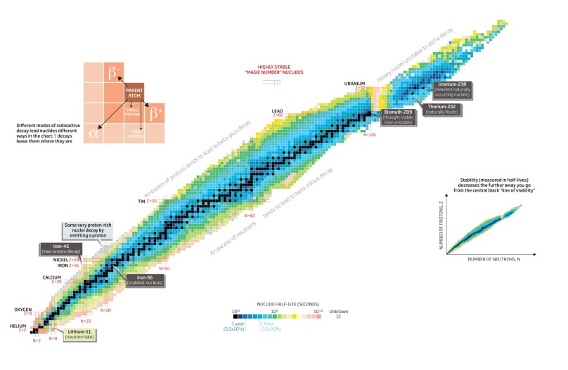
Figure 1. The dynamic well-existence of nuclei. The number of protons is the y-axis and the number of neutrons is the x-axis. http://www.nuclear-power.net/wp-content/uploads/2014/12/nuclide_chart.jpg?11abca

Perhaps I am continuing to commit the error of ignoring the fact that parallel sympositions are also serial. Let’s consider the exact moment an episodically well-existent symposition, Jupiter perhaps, came into the World. If we try to do so, we quickly see that the exercise is rather arbitrary and probably futile; as recently as 1994, the comet Shoemaker-Levy 9 sank into Jupiter, increasing its mass as many others had before it since the primordial nebula of the Solar System. Instead, this exercise once again highlights the fact that the serial symponents of an individual fade in and fade out of the World, and a start and an end to its episode may not be identifiable even if the episode itself clearly is. It may not be clear when a symposition began rolling into a well, unlike whether it did so at all.

Sympositions can be further divided into two classes based on repetition inside their serial partonomy. Frozen sympositions clearly do not have any repetition inside their serial partonomy.³ Unfrozen sympositions with frozen parallel partonomies may, however. Take the Earth-Moon system; its parallel partonomy is frozen as {Earth, Moon}, but every month there is a cycle of poses that repeats itself. I call a sequence of serial symponents that repeats itself a sem-loop and refer to the symponents as being sem-looped or having a sem-loop. Incidentally, the Earth-Moon system is caught in a potential energy well; it is merely cycling around the bottom rather than being stuck there. The Earth-Moon system has a continuous sem-loop, but some sem-loops are discrete, and I will explore that more in Part II.

Since sympositions stack on each other up the levels through the Logos, the ones that are both episodically and dynamically well-existent will be the symponents of those that are well-existent on higher levels. But as with gravity creating nuclear-fusing stars, higher level sympositions can also affect well-existences on lower levels. This is true in general: sympositions in partonomic neighborhoods can modify each other’s well-existences based on their interactions both vertically and horizontally. Sympositions that encourage each other’s well-existence can be called cooperative, and sympositions that inhibit each other’s well-existence can be called competitive. It’s better to ascribe cooperation and competition to the well-existences themselves since they may differ in the episodic and dynamic cases. For instance, supernovae affect the episodic well-existence of large nuclei, but do nothing for their dynamic well-existence.⁴ When the dynamic well-existence of one symposition cooperates with the episodic well-existence of another, it could be stated in more conventional terms that the former causes the latter, in a sense of “causation” that is continuous from non-causation to causation rather than binary between the two extremes.

The last point is that well-existences don’t mean the same thing for each of individuals, populations, and distillations. The original definitions were inspired by the distilled case. A distillation can have degrees of episodic well-existence based on how many individuals matching it that there are, where those degrees lie on one dimension because counting happens on the one-dimensional number line. A distillation can also have degrees of dynamic well-existence, and those degrees similarly lie on one dimension but instead because time is one-dimensional. An individual, on the other hand, does not have degrees of episodic well-existence but either is or isn’t episodically well-existent, depending on whether it did or did not come into the World. Dynamic well-existence operates the same for individuals as for distillations. For populations, however, to be dynamically well-existent is to continue having new episodically well-existent individuals, even if none of them are relatively dynamically well-existent themselves. For populations to be episodically well-existent is to have a first individual in the population that is episodically well-existent, and is again binary as for individuals unlike distillations. Thus distillations and individuals are alike in the dynamic case, and individuals and populations are alike in the episodic case.

Footnotes

1. An exploration of that would require quantum mechanics. If you’re curious, look up Feynman diagrams.

2. The ray is actually slightly deviated so as to favor slightly higher numbers of neutrons than protons. The deviation would be less if electromagnetism was even weaker compared to the residual strong force than it actually is.

3. Well, there is the moment-by-infinitesimal-moment repetition, but nothing on a higher level in the serial partonomy.

4. It’s also possible that one symposition’s well-existence can affect another’s while not having its own affected it all. Such interactions where only one benefits are commensal and where only one is harmed are amensal. The last case is parasitism, where one is harmed by the well-existence of the other while the other simultaneously benefits from the well-existence of the first.

So far, I have not explicitly juxtaposed time with space in the context of symposition, and consequently the concept of sem-linking has by default referred to the collecting of symponents in a region of space at some specific moment. Sem-linking does not have to be restricted in such a way and can collect symponents that have spatiotemporal instead of just spatial pose. {volcanic eruption} is a symposition that is not localized at one specific moment, as is {butterfly} with its splendid metamorphosis. There are two things fundamentally different between time and space that complicate the generalization of symposition to the temporal dimension, however. First, note that if space was 2D instead of 3D—a plane instead of a volume—and was similarly occupied by point-like physical primitives, then the symposition of these primitives into a Logos would be basically the same process as if it was 3D. This holds also if space was 4D and again occupied by point-like physical primitives. The problem is that physical primitives are not point-like in our 4D spacetime; they are line-like, tracing extended paths through the dimension of time.

The other difference between time and space is that, given a bunch of points in space, there is no natural ordering to them, they’re just all there at once. On the other hand, given a bunch of points in spacetime, there is a natural ordering to them: the chronological order of first to last point.¹ A consequence of this is that when a partonomy is serialized in order to put it into writing, for example with a hydrogen atom: {e, {q_u, q_u, q_d}}, arbitrary choices must be made to put the electron before the proton and then the up-quarks before the down-quark. These choices are not arbitrary with the temporal symponents of a symposition; just put the first one first. Consequently, a clear distinction can be made between serial sympositions, whose symponents can be organized temporally in a series, and parallel sympositions, which are sympositions as originally conceived at a given moment of time whose symponents appear together in parallel.

Now, what is the partonomy of a serial symposition and how might it be different from the partonomy of a parallel symposition, and what happens when these partonomies are put together? First, let’s consider a symposition that for at least some stretch of time has parallel symponents that do not move—our atom of hydrogen, perhaps, at a temperature of absolute zero—and we can say that such a symposition is “frozen.” The self-same parallel configuration of the hydrogen atom is present at each snapshot of time, such that there is a series of {e, {q_u, q_u, q_d}}, {e, {q_u, q_u, q_d}}, {e, {q_u, q_u, q_d}}, etc., that is ordered by time non-arbitrarily. Thus it is also a serial symposition. All frozen parallel sympositions are also serial. How can all of these identical only-parallel partonomies be fit into a single serial+parallel partonomy? There is a range of possibilities with two extremes; we can serially sem-link at the Dust or at the top—either as {{e, e, e, …}, {{q_u, q_u, q_u, …}, {q_u, q_u, q_u, …}, {q_d, q_d, q_d, …}}} or as {{e, {q_u, q_u, q_d}}, {e, {q_u, q_u, q_d}}, {e, {q_u, q_u, q_d}}, …} or in between as {{e, e, e, …}, {{q_u, q_u, q_d}, {q_u, q_u, q_d}, {q_u, q_u, q_d}, …}}. They have, respectively, four, one, and two ellipses (…), two extremes and one intermediate, corresponding to the number of nodes at each level.²

Recall that a parallel partonomic gap, if sufficiently large, results in the level below the gap relating quasi-continuously to the level above the gap. The ellipses in the previous paragraph represent serial partonomic gaps, but how large are they? The fact that primitives are lines in spacetime means that they are continuous and that there are infinitely many points between any two moments of time.³ The serial partonomic gap is so large it’s infinite. Whereas parallel partonomic gaps only approach continuity, serial partonomic gaps can actually get there, and this holds regardless of at which parallel partonomic extreme of bottom or top or where in-between the snapshots are serially sem-linked. So what is the spacetime partonomy of a symposition? A final answer requires choosing a level where the serial sem-linking occurs. Such a choice seems arbitrary, however, at least for frozen sympositions, so I won’t make it, instead preserving the tension.⁴ Regardless, we can see that serial sem-linking in frozen sympositions is always continuous.

Two questions related to each other arise. Can there be continuously serial sympositions that are not frozen? And what would it take to have a discretely instead of continuously serial symposition, which of course could not be frozen? For a symposition to not be frozen, poses must be changing somewhere in it over time. Recall that a symposition is more than its partonomy. Though frozen sympositions clearly also have frozen partonomies, sympositions with frozen partonomies do not necessarily need to be frozen themselves. Take the Solar System. The partonomy of the Solar System, at least considering only the planets and the major moons, has not changed in millions years. Still, the earth and the sun have completed millions of loops of a continuous sequence of poses since then, and similarly all the other planets and moons. Importantly, if we tried to discretize the sequence of poses, we would have to make arbitrary choices.

When would we be able to make a non-arbitrary choice? Consider a planet that is happily orbiting the Sun until an unfortunate confrontation with another object throws it off course indefinitely into a highly eccentric orbit. This is hypothesized to have actually happened in the history of our Solar System to “Planet Nine,” which started out between Saturn and Uranus but was at some juncture deflected by Saturn towards Jupiter and then by Jupiter into the far reaches of the Solar System to live out its life with an orbital period of 10,000 to 20,000 Earth-years.⁵ A non-arbitrary division can be made in the temporal series before and after the planet’s deflection. The exact moment of the division may not be easy to determine, but the more important and fortunately easier question is whether there should be a division, and the answer is yes. Regardless, note that the Jumping-Jupiter scenario, as it’s referred to in astrophysics, did not change the parallel partonomy of the Solar System at any moment;⁶ its partonomic relevance is purely serial.

Imagine instead a spaceship that orbits Earth many times and then changes course and orbits Mars many times. The change in course affects the serial partonomy just like above with a clear before and after, but if we construct the parallel partonomy, we see that it is also affected, unlike above with Planet Nine. It goes from {{Earth, spaceship}, Mars} to {Earth, {spaceship, Mars}}.⁷ Let’s continue with just the initial letter of each and try to construct a full spacetime partonomy. The parallel partonomies at first are the repeated {{E, s}, M}, {{E, s}, M}, {{E, s}, M}, etc., but in the end are {E, {s, M}}, {E, {s, M}}, {E, {s, M}}. If we serially sem-link at the gravitational Dust, then we get {{{E, E, E, …}, {s, s, s, …}}, {M, M, M, …}} followed by {{E, E, E, …}, {{s, s, s, …}, {M, M, M, …}}}. Recall that choosing the Dusty bottom instead of some other level for continuously serial sem-linking is arbitrary in frozen sympositions and in sympositions with frozen partonomies, such as the Solar System in the Jumping-Jupiter scenario. When partonomies are not frozen, however, the choice is no longer arbitrary. If we try to sem-link our spaceship scenario at the bottom, we would need to be able to put {E, E, E, E, E, E, …}, {s, s, s, s, s, s, …}, and {M, M, M, M, M, M…} into a tree. This cannot be done in such a way that reconciles both the initial and final parallel partonomies. We can sem-link at the top, getting {{{E, E, E, …}, {s, s, s, …}}, M, M, M…}, {E, E, E, …, {s, s, s, …, M, M, M…}}}, but we procure a very odd result if we do so: the intrinsic serial partonomy of Earth is sliced in two by an extrinsic spaceship flying to Mars!

We can solve the problem by an analogy with taxonomies. There were two ways in which a taxonomy could fail to be a tree: by the presence of either continuous or cartesian variation. There are also two ways in which a partonomy can fail to be a tree. The first has already been covered above: continuous sem-linking does not provide a tree, nor even a graph, because both of these are discrete mathematical objects. The second way occurs when symponents belong simultaneously⁸ to more than one symposition, a situation that can still be depicted by a graph if no longer by a tree. Non-hierarchical partonomies are ubiquitous. They are necessary any time a symponent moves from belonging to one symposition to belonging to another. Though non-hierarchical partonomies are first defined here for temporal reasons, we will see later that they are also relevant spatially.

Figure 1. A non-hierarchical serial partonomy.

Though we need non-hierarchical partonomies to fully account for it, spatiotemporal symposition is as full of hierarchical possibility as just spatial symposition. Consider the spatiotemporal partonomy of an individual {football game} or individual {conference}; they both have many levels above the lowest discrete serial symposition. I’ve mentioned several times that the Logos has developed, grown, or changed after the Big Bang. Given serial sem-linking, however, those expressions are faulty. The Logos spans all of spacetime, planted firmly on both the primordial homogeneity at the Big Bang and the ever-present Dust. The Logos hasn’t developed after the Big Bang, but rather the horizon of its revelation has been expanding.

Footnotes

1. Ignoring relativistic concerns regarding frame of reference. Again, this book is focused on the classical realm.

2. In {e, {q_u, q_u, q_d}}, there is one level between the quarks and the atom, but no levels between the electron and the atom. The in-between serial partonomy could alternatively be depicted as {{{e}, {e}, {e}, …}, {{q_u, q_u, q_d}, {q_u, q_u, q_d}, {q_u, q_u, q_d}, …}}, for clarity. Also, there’s no need distinguish the serial symponents, with subscripts for instance, because of the direct mapping between the seriality of writing and the seriality of time.

3. You may object because of the Planck time. Note that the Planck time does not set a discretization of time, but rather a bound for the measurability of time. Time could go unmeasurably crazy at such tiny scales even while remaining continuous, if it behaved something like the Weierstrass function or the Koch snowflake, perhaps.

4. The tension can be explored further in the endurantism vs. perdurantism literature, although it doesn’t explore the in-between possibility.

5. http://www.nature.com/news/evidence-grows-for-giant-planet-on-fringes-of-solar-system-1.19182

6. In all likelihood there was a reorganization of moons, but we are entirely ignorant of the details, so I’ll ignore this possibility.

7. Continuing with the theme of a very pruned Solar System.

8. “Simultaneously” in a timeless, 4D sense, perhaps oxymoronically.