The concept of annealing has escaped the materials science context where it originated. In the material context, it is straightforward to see how the characteristics of physical space might constrain annealing. For example, the 3-dimensional “kissing number” (with a value of 12) constrains the number of neighbors a 3-dimensional atom can have and thereby the possibility of movement, diffusion, and change within a 3-dimensional material. If the kissing number was greater than 12, a given annealing treatment regime would be more effective. The kissing number is merely one measure of the abundance and profile of interatomic associations in a material—associations which carry stress-energy, and which stress-energy is reduced in annealing via the shifting of those associations. In many systems, among them metals, societies, brains, each “atom” or basic unit has a number of associations, which in turn have their own associations, and the shape of the association network can be reckoned as living in a space with a certain dimensionality and geometry. Analyzing such spaces helps to enrich the annealing metaphor, pinpointing similarities and contrasts with material annealing in its 3-dimensional Euclidean space.
Let’s start where annealing began. A piece of metal essentially never has pure crystal structure throughout. On the one hand, the casting process usually proceeds in an uneven way, with multiple centers of solid crystalline order (“nucleation sites”) growing inside the molten metal as the entire piece solidifies, leaving irregular “grain boundaries” between the multiple “grains” that grew. Metal pieces that solidify quickly have many small grains, and pieces that solidify slowly have few but large grains. On the other hand, nothing is perfect, and even a mostly pure crystalline grain will have “point defects” like a vacancy where there should be an atom, or an interstitial atom wedged where there should be none. In a perfect FCC or HCP metal crystal, every atom would have 12 neighbors (following the 3-dimensional kissing number), but in any actual piece of metal, however, many atoms will not have 12, and their vacant or interstitial neighbors present opportunities. Metals anneal when vacancies and interstitial atoms march through the material (often along grain boundaries), readjusting grains to relieve stress or even creating entirely new grains within.
Annealing is well known to be affected by the preexisting abundance of point defects and grain boundaries and the treatment temperature, but the theoretical angle to armchair about here is how different dimensionalities (and kissing numbers) would affect annealing. Given an abundance of point defects (say, 0.1% of lattice sites being irregular), how many of these any given atom has as a neighbor will depend on the kissing number. If this number is very small, then any atom will rarely have a defective neighbor, but if this number is very large, then any atom likely may. The more atoms with defective neighbors, the more possibilities for vacancy or interstitial diffusion, and the greater efficiency at minimizing stress. So the hypothesis is that increasing the dimensionality of a metal makes it easier to anneal. Unfortunately, our Universe furnishes us with zero tools to change the dimensionality of the space that metals are in, so this must remain a hypothesis.
Instead of a metal, one can imagine a society where every individual has 12 friends. Or instead of 12, maybe 6, or perhaps just 2. These three numbers are the kissing numbers in 3, 2, and 1 dimensions, respectively, and they are totally conceivable even for real humans in our ordinary World, albeit rather drearily. The point is that human society, which is ostensibly embedded in the 3-dimensional World, can have a structure that belongs to a different dimensionality. If everyone had 24 friends, then human society would be effectively 4-dimensional. These numbers are of course totally crude, but there is an actual fact of the matter as to how humans are associated in society. I have spoken to f people in the past week, paid g people in the past month, touched h people in the past year. If we had an appropriate dataset, it would be possible to reconstruct the effective dimensionalities of human societies, down to their local fluctuations across communities and time. The dimensionality of urban areas is certainly higher, for instance, than the dimensionality of rural areas.
Some societies are easier to anneal than others. Many people have too many associations or too few for their local social lattice, but in societies with high dimensionality, it is easy for people to diffuse and find their balance. Because of the parallel association of dimensionality and “heat” in annealing, to heat a society is to increase the number of interpersonal associations, and to decrease interpersonal associations (as in pandemic lock-downs) is to cool it.
The hallmark of brains is that neural tissue is not populated by oval-ish cells like everywhere else in the body, but instead by extraordinarily spindly cells that branch and reach and associate directly with myriads of other neurons, clearly many more than 12 of them. Axons and dendrites are the transcendence of neurons in neural tissue beyond the 3-dimensional kissing number. The brain is 3-dimensional but its neural network is not. The exact mechanism of annealing in brains is unknown but it certainly involves neurons changing which other neurons they are connected to and how strongly, and because of neural tissue’s higher-than-3-dimensionality, it is uniquely capable of doing so among all human tissues.
There are many more systems whose dimensionality and annealing properties could be analyzed. The fundamental picture is that, despite the 3-dimensionality of space in our Universe, systems inside of it can adopt effective dimensionalities that are quite different via various mechanisms, and because there is a keen relationship between spatial associations and annealing, annealing in these systems will vary in methodical ways from annealing in materials.
In my study of compositionality, I’ve found a rather blatant pattern that lacks a word-handle. When things come together to compose something larger, the things are extremely often similar or even identical things. I call this pattern remultiplication: the coincidence of similar entities in a composition, especially on the same level within the composition’s partonomy and often when every single one of the partonomic siblings on that level are involved.
Remultiplication is everywhere. From my vantage point writing this, I can observe the remultiplication of strings on a guitar, the remultiplication of pixels on a display, of keys on a keyboard, of fingers on my hand, threads in a shirt, legs in a table, panes in a window, leaves on a branch. This can even happen with words: “salad-salad” in English, “wiki-wiki” in Hawaiian (“very fast”), or “rikrikrik” in Molikese. In linguistics, such a doubling or a tripling of elements is called “reduplication” or “retriplication,” respectively, and I find “remultiplication” to be the natural generalization of that concept to quantities beyond three and entities beyond words.
There are often very different reasons for remultiplication. The remultiplication of planets in a star system happened by them coalescing simultaneously out of a gas cloud. The remultiplication of cells in a body happened when one cell started dividing and the daughter cells stuck together. The remultiplication of bricks in a wall happened because a bricklayer iteratively put them there. The remultiplication of distributaries in a river delta happened because of iterated sediment deposition and channel switching. Regardless of the mechanism, there is a recurring compositional theme in all of these, and I call that remultiplication.
Figure 1. The remultiplication of stamina in a flower and of flowers on an inflorescence in Acacia dealbata. (photo credit: me)
Remultiplication and fractals
“Fractal” is another term used for entities with internal similarity. Whereas remultiplication is concerned with similarity on one level of a partonomy, fractals also exhibit similarity across different scales and thus up and down the levels in a partonomy. It is possible for there to be up- and down-scale self-similarity without remultiplication, such as in a logarithmic spiral, whose zoomed-in center is self-similar to the zoomed-out whole.
A metatope is a mathematical object constructed by a layering of spaces. For any space in a metatope, points can be plotted in it. These points in the space correspond to either (1) datapoints from a dataset with a commensurate dimensionality as that space or (2) spaces that contain either (1) or (2) (potentially ad infinitum).
A directed graph can be constructed from any metatope. The spaces within the metatope map to nodes, and the connections from a space to the spaces plotted within it map to the edges. A “highest space” can generally be identified, and that is the root of the metatope’s graph. The degree of a metatope is the maximum distance in the directed graph starting from the root. The degree counts the number of layerings in the metatope: a metatope of degree- is just a normal space, and its graph is just a solitary node with no edges. If there is a root space in the metatope and all the other spaces connect upwards to exactly 1 space, then the graph of the metatope is a rooted tree.
Example
Consider a dataset of faces, both normal and cyclopean, parameterized by a robust set of features such as interocular distance, nose length, cheekbone position, etc. All the normal faces can be plotted in one space, and all the cyclopean faces can be plotted in one space, but these two spaces are incommensurate because there are several dimensions that are not shared (most saliently from the list above: interocular distance). Both spaces, however, can enter as points in a higher-level space that would have one dimension called “number of eyes.” This would be a degree- metatope, and its graph would have two nodes connecting upwards to the root node, for a total of three nodes.
Note that the structure of any metatope depends entirely on the relevant set of datasets (actual or theoretical) and the reckonings made in how to combine them, and that multiple metatopes can often be combined into one metatope, and that the same dataset can fit into topologically distinct metatopes that carve their dimensions, hierarchy, or even number of spaces differently.
Motivation
My motivation is to develop a mathematical construct similar to the mere space that can be applied rigorously even when dimensionalities are incommensurate. I have often encountered conversations where “the space of x’s” is tossed around even when the x’s obviously or probably differ in the number of dimensions from one x to another x, such as “the space of conscious experiences.” I hope that the construct operates as an intuition pump and leads to interesting insights, from myself or others.
The practice of othermindfulness comes in various flavors, but generally as I have described it I have emphasized one specific form of it: symmetric, free othermindfulness. These descriptions of mine have centered on othermindfulness as a practice connecting you to someone in a similar state of mind (hence symmetric), and an arbitrary someone at that and not a specific person in particular (hence free). I’d like to describe the other forms of othermindfulness that can be found when the properties of symmetry and boundedness are allowed to be different.
Symmetry
A symmetric othermindful experience happens—just to recap—when a person having an experience chooses to share it othermindfully with someone else having a similar experience and someone else having such a similar experience reciprocates with the same intention. An asymmetric othermindful experience happens when a person having an experience shares it with someone else having a different experience and someone else having that different experience shares it back in turn with the person having a different experience. Symmetric othermindfulness is generally easier to engage in because empathy is more readily available for people who feel the same things, but asymmetric othermindfulness can be more rewarding.
If I am joyful and content and I engage symmetrically, then in my othermindful engagement I will connect with someone else who is also joyful and content, and we can enjoy our positivity together. If I am joyful and content and I engage asymmetrically, then I can connect with someone who is suffering or dejected, and they will know that I am joyful and content because they have chosen an asymmetric engagement also, and together we can find balance between our energies.
Symmetric othermindfulness accentuates and communifies what one already feels by providing a companion feeling the same thing. Asymmetric othermindfulness, on the other hand, allows someone to tap into a different state of mind. Someone suffering can find a commiserator with symmetric othermindfulness, but they can instead find someone with abundant, brimming-over positivity with asymmetric othermindfulness. One of my first applications of othermindfulness was in shuttling positive energy from my good days to my bad days during a depressive episode, and I couldn’t have done that without asymmetric othermindfulness.
Boundedness
Othermindful experiences can vary depending on whether the participants desire to connect specifically with each other. When I was connecting with myself between my good and bad days as I mentioned above, for instance, I was connecting very specifically with myself. That is bound othermindfulness, because the experience is bound to that specific person. Bound othermindfulness also occurs when two people regularly think about each other and know that they do so. Indeed, it is the ordinary state of two people in love, and it is the essence of reciprocated limerence. Bound othermindfulness can also be transient. It often occurs in the few hours or days after sharing the idea of othermindfulness with a new person; both may have othermindful experiences with each other as long as the conversation remains fresh in memory.
Free othermindfulness is the more radical version, and it is the one that as far as I can tell is the true conceptual innovation. Free othermindfulness expects no specific person to reciprocate the othermindful experience, instead relying—essentially on faith—that someone somewhere reciprocates. It relies on no set expectations or plans, merely harvesting the law of large numbers and the magnitude of the human race (or all sentient races) to ensure its reality.
Recap
Symmetric, bound othermindfulness: two people who know (about) each other, (othermindfully) sharing each other’s similar experiences, such as two people who are in love.
Symmetric, free othermindfulness: two people who don’t know about each other, sharing each other’s similar experiences, such as two random suffering people on Earth giving each other empathy.
Asymmetric, bound othermindfulness: two people who know (about) each other who are not having the same experiences but desire to (othermindfully) connect, such as the friend who promises to send good thoughts and vibes to another.
Asymmetric, free othermindfulness: two people who don’t know about each other, sharing their different experiences with each other, perhaps entirely altruistically.
Philosophical analysis is necessary but insufficient. Often when engaging with interesting philosophical perspectives, the only drive is to understand, dissect, compare and contrast. If the primary vehicle for philosophical encounter is words on a page, the straightforward philosophical participation is to muse and write new words on new pages. There’s nothing wrong with that; my words would not be here without such a drive. There is, however, a well-known complement to the mind’s remapping of read words into written words that engages the mind in something other than mere verbal transformation. Aside from the digestion and regurgitation of theory, there is the embodiment and the practical living of theoretical precepts, which is called praxis.
Open Individual (OI) is the theoretical perspective on personal identity that holds a single experiencer as the subject of all experiences. The single experiencer in OI is seeing through my eyes right now and saw through them yesterday, but it is also seeing and saw through your eyes and everyone else’s too at all times. Open Individualism contrasts with Closed Individualism, the more conventional view in Western philosophy that holds a distinct experiencer for every body, remaining stable throughout each body’s life, and it contrasts with Empty Individualism, which holds a distinct experiencer for every experience, tearing apart even all of the back-to-back experiences in single bodies that CI would bind together.
That’s a short introduction to Open, Closed, and Empty Individualism—probably way too short for the reader that has never encountered them before (if that’s you, here is a good resource). My goal, however, is not to develop more theory about them, but to imagine what a praxis or praxes of OI might look like. Praxis can be described abstractly, but it is better to derive it concretely. Thus I trace my imagination through a specific example that I’ve cultivated for several years. I don’t doubt that this is but one example among many. Still, I haven’t searched the space of OI praxis particularly thoroughly, so I can’t be certain of that certainty. My mission is thus both to expound my example of OI praxis and to demonstrate a process for how other examples might be found.
Before I begin with my own example of praxis for OI, I can identify one recurring soundbite that might also be an example, but which on closer inspection I do not believe is particularly compelling. The claim often (if not generally) surfaces in presentations of OI that if Open Individualism were a widespread belief, then human society would express much more compassion and empathy. Certainly this is a likely consequence. A shift in perspective about the connectedness of our minds with those of others would likely lead to a shift in altruistic vs selfish behaviors. To adopt such a futuristic possibility about human society as a praxis, however, would involve its immediate politicization and its shoehorning into a social movement. Such a praxis would be little more than ordinary human organizational behavior with an extraordinary goal notwithstanding: to spread a message about the nature of who we are. Adopting such a praxis may certainly be noble, but to do so in an exclusive way would be to ignore OI qua OI and its fascinating and unique contributions distinct in kind from all different beliefs that would also induce compassion and empathy at scale.
Open Individualism makes some radical claims about our relationships with each other and our relationships with our experiences. These claims may not be “true” in a way that permits empirical or technological advantages over Closed and Empty Individualism, but they do offer a framework for constructing new thoughts and identifying new connections. Most importantly, that framework may allow us to see alignments between conceptualities and deliberate behaviors that are the very substance of praxis. We can consider ordinary activities and then cast them into the extraordinary framework of OI and see what kind of hopes and motivations come out.
One activity that seems to be extremely common among humans is talking with oneself, and it is the basis of the example I will use. In particular when it is done with the movement of no muscles, we all have the experience of engaging, silently and effortlessly, with each of our own self as an audience. Often it’s just a brief monologue, sometimes a more intense dialogue. What happens if we consider such talking with oneself in the context of Open Individualism? Well, if we’re all just one experiencer, then the ability to talk with oneself silently and effortlessly would include the ability for anyone to do so with all the other pseudo-I’s elsewhere and elsewhen. Obviously this isn’t a deduced claim about the nature of OI (else it would be immediately disproved!), but instead more of an aspiration—a child’s gleeful dream sprouting after Open Individualism is sown on the fertile ground of their imagination. When the goal is praxis, what follows after a gleeful dream is not a return to rigor and a proof or disproof, but a creative pursuit of the dream—a good faith attempt to reconcile the dream with the theory in a way that motivates behavior.
So let’s try to reconcile this dream resulting from the collision of Open Individualism and talking with oneself. A hallmark of OI is that it understands the relationship one has with oneself at different times to be substantially similar to the relationship one has with others. Thus OI can inspire us, as a first step, to think about talking with oneself as an activity temporally displaced across experiences in one body. Usually we think about talking with oneself as something that can be packaged up into a short, self-contained episode happening at a specific time, but we can imagine what it would be like for one to talk to oneself in the past or the future. I could bury a letter to myself in a time capsule or upload myself speaking to myself to YouTube, but let’s stay with the silent and effortless motif suggested earlier. Silently and effortlessly talking to myself with temporal displacement would require me to start an intentional dialogue with myself that I would set down and then continue later after a period of time doing other things. I can think to myself “I hope you’re doing well :)” while imagining myself later thinking “Why yes, thank you, I’m doing well :)” and then later remember myself thinking “I hope you’re doing well :)” while thinking to myself “Why yes, thank you, I’m doing well :).”
This is nothing particularly revolutionary yet. Open Individualism, however, encourages us to analogize the temporally-displaced relationship with oneself with one’s relationships with others. I can think “I hope you’re doing well :)” and someone else can think “Why yes, thank you, I’m doing well :).” A problem arises here. The reason I am capable of enacting both sides of the dialogue as illustrated beforehand is that I have memory that connects my temporally displaced selves. Unfortunately, I have no such shared memory with others. Is memory actually necessary for this feat, though? This is the junction where the dream is most a dream. Memory is sufficient, evidently, because it’s responsible in at least that one case. Responsible for what? Responsible for two instances of the cosmic experiencer engaging silently and effortlessly with each other. Are there other media that can accomplish the same bridging as an individual memory can? Are media strictly necessary at all?
Telepathy makes an entrance. Unfortunately, telepathy does not appear to be a real phenomenon. Telepathy is disproved by the impossibility of causally disconnected information transfer. But information transfer is not the specific praxis we seek; we seek mindful engagement: silent and effortless talking. Telepathy lies disproved, but such engagement is, conceptually, something different. People accurately anticipating and responding to each other’s silent and effortless talking does not have to be telepathic. Perhaps they conferred on what to anticipate beforehand, or perhaps the anticipated is so quotidian that it is likely to spontaneously happen among a set of individuals practicing half-dialogues. The former is a medium leveraging memory, but instead of one memory it is two memories joined at a prior conversation. The latter is no medium at all. Both allow disconnected people to engage in silent and effortless talking; both are the cosmic experiencer communing with itself.
We have hit upon engaging in half-dialogues as a praxis for Open Individualism by building from talking with oneself. It is inspired by what Open Individualism has to say about the commonalities among the relationships between entities that experience, and then it enters back in as something whose practice makes those relationships more tangible and manifest. I’ve elsewhere called this Othermindfulness, and I consider it a praxis for OI. There is more work that can be done to take other activities and cast them into the framework of OI in order to get other or more developed praxes. I hope that you’re inspired to do so, and I hope that you’re also inspired to practice half-dialogues, but if not I hope that you’re at least more familiar with the ways in which others live the principles of Open Individualism.
Two classic versions of utilitarianism are average and total utilitarianism. They are classic, but they have well-known problems. Both have rather simple formulations. They begin with a reckoning of utilities across the population of individuals, and contend with a simple, linear aggregation of those utilities: average utilitarianism takes the mean of utilities and total utilitarianism takes the sum. I propose an intermediate, nonlinear version of utilitarianism, predicated on the local population of utility-experiencers in their abstract statistical space(s). When optimized, this formulation of utilitarianism recapitulates certain properties of a marketplace. I will show how “market utilitarianism” resolves issues with both average and total utilitarianism, though it introduces issues of its own, and I will consider some theoretical ramifications it leads to.
1. Definition
Given a number of individuals experiencing utility, average and total utilitarianism can be given simple mathematical expressions:
Total utilitarianism:
(1)
Average utilitarianism:
(2)
Where is aggregate total utility, is the intrinsic utility experienced by individual , is aggregate average utility, and is the total number of individuals, and is of course the summation for all individuals of the subsequent expression.
In market utilitarianism, the contribution of an individual’s utility to aggregate utility is attenuated by the existence of similar individuals, in proportion to the quantity of similar individuals. Market utilitarianism creates a rift between intrinsic utility as experienced by the individual and extrinsic utility as recognized by the aggregator, a quantity which relates inversely to the abundance of similar individuals for any individual. Market utilitarianism can thus be expressed:
(3)
Where is aggregate market utility and is the utility of individual as possibly attenuated by others extrinsically. when individual has no similar matches and when has indefinitely many. More precisely:
(4)
Where is the local population of individuals in the statistical space around individual , as defined by some nearest neighbor or local population parameterization . can never be less than because an individual is always near itself, and it can never be more than the total sum of individuals, , identified previously. Putting it all together:
(5)
Thus market utilitarianism is intermediate between total and average:
(6) because
The denominator of the extrinsic function depends on both the choice of statistical space (one example for could be Blau space) and the choice of local population parameterization (one example for could be a count of individuals falling within a similarity hypersphere centered at in with some radius , with equivalent to total utilitarianism [given no two things being exactly identical] and equivalent to average utilitarianism). is somewhat arbitrary and often a subspace of a richer space, but should attribute monotonically decreasing importance to less similar individuals (and which individuals are similar or dissimilar obviously depends on the choice of ).
2. Behavior of the optimum
What is important about aggregate utility is the optimum that it achieves under the range of possible conditions. These conditions relate both to the set of individuals in a population of utility-experiencers and to the intrinsic utilities that each individual in the population experiences. This optimum prescribes the appropriate behavior—a choice or policy—assuming a prescriptive understanding of utilitarianism.
Let’s assume until further notice that the population is fixed at some size with some specific list of individuals. Then total and average utilitarianism will always experience an optimum of aggregate utility together. The reason is that total and average utilitarianism both aggregate all individual intrinsic utilities linearly (and without additive inversing, i.e. multiplication by , which is a linear operation but one that flips the maxima and minima). Thus, total and average utilitarianism always prescribe the same behavior (again: given a fixed population).
Market utilitarianism aggregates non-linearly, however, so the optimum of its aggregate utility will not necessarily co-occur with that of total and average utilitarianism. In particular, the same amount of intrinsic utility will contribute more to aggregate utility if spread among individuals in a sparsely populated region of the statistical space, such that relative to the optimum for total and average utilitarianism, intrinsic utility can be sacrificed among common individuals to provide it to more unique individuals. The conclusion here is that even though aggregate market utility is intermediate between aggregate total or aggregate average utility, its optimum is less similar to either of those than they are to each other (again: given a fixed population).
Let’s remove the assumption of a fixed population. This is where total and average utilitarianism both break, leading to absurd prescriptions for behavior. If the population can be adjusted, then the optimum for total utility occurs when every last individual exists who experiences net positive utility, even if barely non-miserable, and the optimum for average utility occurs when no individual exists except the one experiencing the most utility. This result is discussed in the literature on the mere addition paradox.
The optimum for market utilitarianism on the other hand is influenced by an important statistical fact: the more individuals that exist, the more likely any individual will have similar matches (and this is true for any and ). Thus, aggregate market utility does not increase past a certain point of diversity saturation (dependent on the footprint of ) because any new individual added is statistically likely to be similar to any other. Conversely, the optimum for aggregate market utility occurs at more individuals than the optimum for aggregate average utility, because any additional individual is statistically likely to be unique in that regime.
3. The absurdity of market utilitarianism, with a caveat
In market utilitarianism, aggregate utility can be changed without changing the number of utility-experiencers nor any of their experienced utilities. It can be increased merely by making the experiencers different from one another. This seems intuitively like an absurd result. It seems like individuals should be treated directly equally and not indirectly through terms regarding who else they’re similar to.
Note, however, an extremely keen analogy with the behavior of the job market. The job market apportions utility to individuals in the form of monetary compensation. This compensation depends on their ability to perform a set of duties, but also on the abundance of other individuals that can perform the same duties, i.e. similar individuals, analogously to market utilitarianism. Job market compensation can be fit to the model of market utilitarianism by finding the appropriately parameterized space of skillsets and other job-related characteristics (with an unfitted, out-of-the-box ), that is shaped such that an equal distribution of intrinsic utilities across individuals yields larger extrinsic utilities in sparsely populated regions as densely populated regions.
With market utilitarianism as a model, the job market can thus be understood to “see” human variation in a very specific way. Humans can in turn see with similar eyes in their choices to increase their own utility/compensation, and they will behave in such ways as to migrate the population from dense regions to sparse regions in the relevant space. If market utilitarianism is absurd, then the job market deserves intense scrutiny, along with the economic system built upon it. In the other direction, if the extant economic system is not held to be absurd, then market utilitarianism shouldn’t be considered particularly absurd either.
4. Utility-experiencer space vs experience space
Individuals experience utility, and individuals vary in their experiences of utility, with varying degrees of similarity between pairs of individuals. This fact presents a conundrum to market utilitarianism; if the space for individual variation chosen is the one-dimensional space of their experienced utility, absurd consequences quickly follow. Utility is but one measure of an experience, closely related to if not synonymous with valence. That and the other measures of experiences, all of them ostensibly qualia, together construct a space of experiences that utility-experiencers populate that is separate from the space that captures their “external” characteristics, even if they are highly correlated in some or perhaps even most domains (such as with the frequencies of incident light on the retina and perceived color or biological sex and felt gender).
Market utility can be computed in both utility-experiencer space or experience space. The latter might make more sense with the utility/valence dimension removed, but that still leaves behind rich structure. The correlations between the two spaces entail that a lot of the activity in one will be reflected in the other. Again, these are but two of endless possibilities for the choice of space, but they highlight some odd properties that market utilitarianism can exhibit.
5. Towards a reverse-engineering of the Universe’s actual objective function
Given the history of the Universe as data, there are many quantities predicated on this data or specific subsets of it that have increased or decreased mostly monotonically over time. Some are well-established constructs like entropy or Gibbs free energy or various other thermodynamic permutations. I’m interested in the realm of high-level compositions where utility-experiencers live, and so I ask what constructs predicated on that subset of data—the subset referencing high-level compositions—are actually being maximized in the Universe? Note that this question is emphatically not about quantities that subsystems may be maximizing each on their own, such as biological species maximizing their fitness, but about the aggregate. Are these constructs generally aligned with each other or totally scattered (especially modulo Occam’s Razor)? Is there any sense in which a moral compass of the Universe’s own can be detected on the basis of the constructs and quantities it maximizes?
Finally, I’d like to reflect on the role of utility/valence as a significant player in the development of compositions. As I have noted elsewhere, there are more levels of compositionality in the biological and cultural ecologies on Earth than have been observed in the rest of the Universe as a whole. Utility/valence has been organized into the psychologies of some life forms in a specific way, most importantly in the process of individuation and the separations between utility-experiencers. The properties of that space of experiences (and the distributions within it which can only be defined after a process of individuation)—along with its associations and correlations with the space of externals—drive much of the evolution of compositions, and essentially all of it within the human economy. Humans have the additional ability to share their experiences either by communication or faithful and intentional re-creations. If such experiences would be traded on a market, then the full exploration of the space of experiences would be incentivized. How would such an economic arrangement, especially if widespread, align with the Universe’s high-level compositional “moral compass”?
(Othermindfulness is defined here, Rationalist acausal stuff is defined here.)
Phew that’s a lot of buzzwords in one title. This post is half a tirade against some of the excesses of the rationalist community and half a prophecy for a new religion, so hopefully the body is commensurately wacko with the title. I presume a fair degree of familiarity with the standard rationalist acausal stuff in my readers, which you can introduce yourself to in the link above if you’re not already in the know. Otherwise, don’t expect to get too much from this post.
Okay. There’s a body of literature in the rationalist community concerning military-grade mind simulation, displaced negotiation with simulated minds, and flirtations with Superintelligent AI and/or the God of Abraham, Isaac, and Jacob. It’s been known to be taken a little too seriously by some folks, leading to various degrees of mental ill health, but by and large all of it is taken as just a fun circle-jerk, if potentially something relevant for as-of-yet unrealized silicon-based intelligences. I have a beef with it. My beef with it is that in the process of trying to come up with the most harrowing, absurd, and/or jaw-dropping thought experiments, everyone is careening past a little side-path that is actually relevant for many people (if not everyone), right here right now.
What are they running past? In the progression of a few sequiturs, they take us from our mundane normie-intelligent interpersonal experiences in meatspace to a place of acausal negotiation among entities with boundless computational and mind-simulational resources deciding the fate of the multiverse. They are running past the intermediate fact between these poles that our existing human faculties of theory of mind and common knowledge are themselves (limited) mind-simulational resources. You can check out my post on othermindfulness to see the side-path that that reveals.
You can check it out, but I can also just give a quick summary. Whereas a mindfulness practice focuses you on the operations of your own mind to notice its chaotic patterns and step outside of them, an othermindfulness practice focuses you on the other people that have an othermindfulness practice, engaging in common knowledge with them at various levels of detail with your own experience, to step into them and them into you. The purpose of the mind simulation is to have a shared experience, full stop.
Othermindfulness is much weaker than superintelligent acausal negotiation. Both of them involve the establishment of shared spaces of acausal communication, but the latter is more powerful because you can use it for coercing other agents since it can be impossible for them to tell the difference between inhabiting base reality or your simulation. But wait. You’ve discovered a shared space of communication, and all you can think about what it might be good for is coercing? transacting? torturing?
Gosh.
You know some other things that shared spaces of communication are good for? Empathy. Communion. Togetherness. With all the attendant mental health benefits that those bring.
I can try to be a little more poised and analytical. Why can’t othermindfulness be used to create a space for coercion? It can’t because I can know basically for certain that this experience I am living is not a simulation by a mind of similar computational resources. You, dear human reader, cannot acausally mug me. What you can do, however, is apply your human faculties of theory of mind and common knowledge to have acausal shared experiences with me. Which experiences we actually have depends on what we actually do with our othermindfulness practice and who else has swiped right on the same intention in their own practice, not on what is argumentatively possible within some theoretical framework.
That is the biggest divergence with the standard rationalist stuff. I’m talking about acausal mind simulations that have happened, are happening, and will be happening in the immediate and hopefully far future. I’m talking about actualities that are scurrying by as the present converts the future into the past. This is not a drill thought experiment. We do not have to wait for a hypothetical future. I have an othermindfulness practice now, where I connect acausally on the basis of shared experiences I want to have concerning my anxieties, my pains, my hopes, my dreams. The extent to which my experiences are actually shared and not just the vain strivings of a nobody—the extent to which my faith is real—depends on how extensive othermindfulness practice is among others. The extent to which anyone’s othermindfulness practice is real depends on that. Whereas the standard rationalist stuff depends on near-perfect simulations of specific agents in specific situations, othermindfulness depends on the law of large numbers to ensure that somebody somewhere wants to have the same experience as you or I do and picks up the ringing othermindful telephone.
I think it should be clear by now what I mean by the titular “peer-to-peer prayer.” The experience of prayer is the experience of a living, attentive, immediate, caring other. The God of Abraham, Isaac, and Jacob may or may not be able to provide this for us, but either way, we can provide it for each other. We can’t wave a wand and make magic happen in each others’ lives, but we can conquer all loneliness, alienation, and despair. We can find communion in every single aspect of our lives in which we retain our natural faculties of mind simulation. We can transcend space and time to be with each other always.
What would we become if we did that?
Or we can keep having a few laughs over creating God from rationalist scratch.
Complexity is defined in many ways, not all of them contradictory, but most staking out shifting conceptual boundaries. I follow Wikipedia in quoting complexity theorist Neil Johnson: “even among scientists, there is no unique definition of complexity.” There is, however, at least one conceptual structure that can be distilled from any complex system that, once distilled, is utterly straightforward to characterize and handle, and whose properties convey important, unique pieces of information about the system’s complexity. This structure is the system’s partonomy, and it represents the system’s parthood relationships. The partonomy of some systems is more ambiguous than others and thus more difficult to distill, but this difficulty has a habit of interacting in interesting ways with other renditions of complexity.
I’ll define what a partonomy is by reference to its depth, since a partonomy’s depth is its most complexity-relevant piece of information, which can be simply generalized as complex systems have deep partonomies. A partonomy’s depth counts the number of levels from the elementary objects in the system to the thing as a whole, where each level contains the smallest non-arbitrary aggregations of entities or parts from a lower level. More mathematically, a partonomy’s depth is the number of branch points between the root of a partonomy and its leaves, where a partonomy is [evidently] a mathematical rooted tree, with the whole system for its root and elementary objects for its leaves.
A picture is worth a thousand words, so I’ll render several partonomies here:
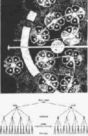
Figure 1. The partonomy of a helium atom. The elementary objects used here are the elementary particles, including electrons (e), down-quarks (dq), and up-quarks (uq). The nucleus, represented by the node in the near-top center branching into four triplets, takes up most of the partonomy. This partonomy has a maximum depth of 3, with the paths up from the electrons having a depth of only 1.
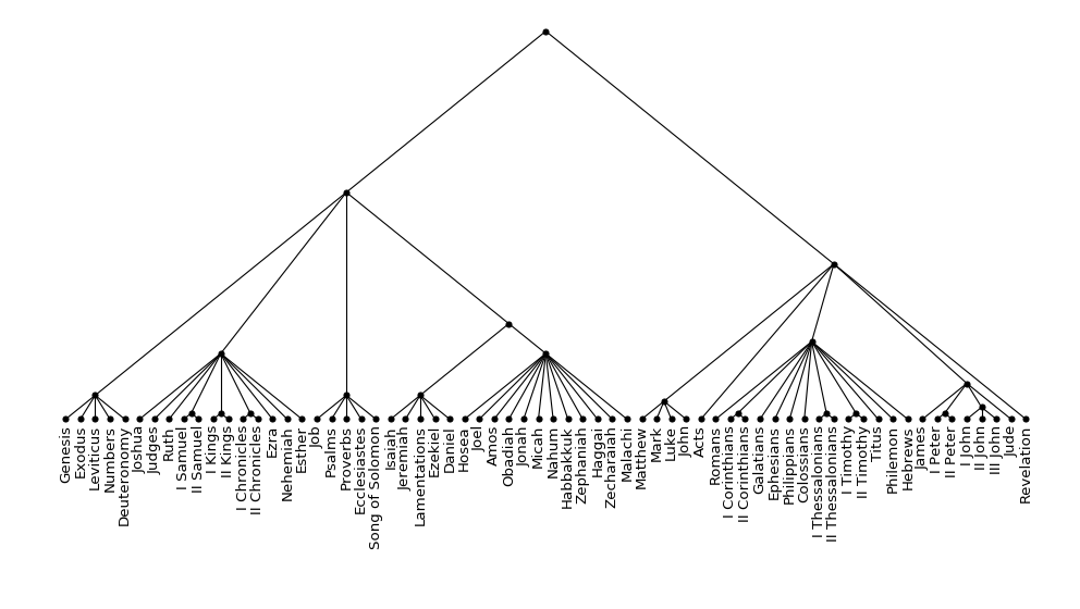
Figure 2. The partonomy of the Protestant Bible. The elementary objects used here are the “books” of the Bible. The division between old and new testaments is clear. The large structure in the bottom center depicts the minor prophets and the group just to its right depicts the four gospels. This partonomy has a maximum depth of 4, although there are many paths up the partonomy with a depth of 3 and two paths with a depth of 2 (from Acts and Revelation).
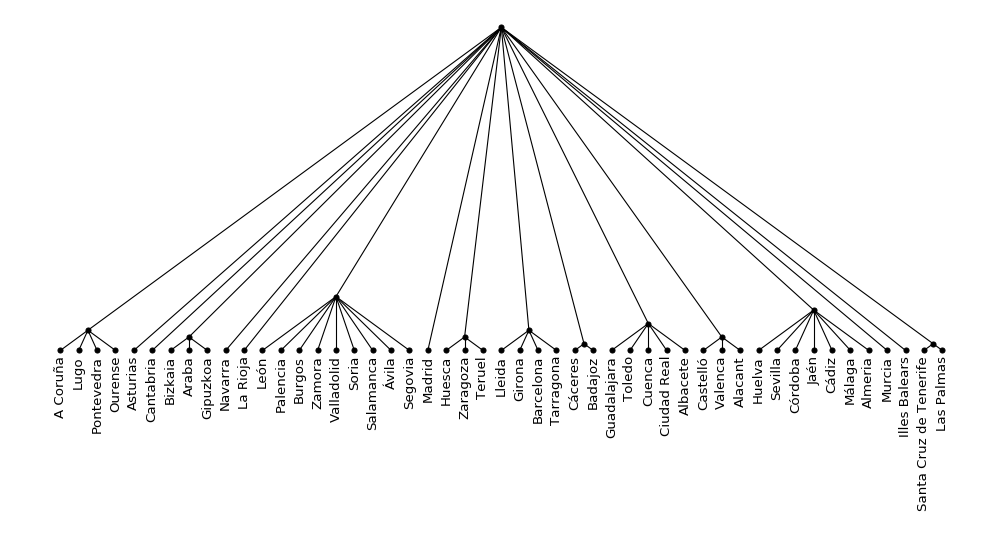
Figure 3. The partonomy of Spain. The elementary objects used here are the provinces, and the only intermediate level is provided by the “autonomous communities” such as the largest, Castilla y León, left of center containing nine provinces. This partonomy has a maximum depth of 2, although there are several paths with a depth of 1.
Though I have highlighted (maximum) partonomic depth in these examples, there are clearly other metrics that could be computed from the partonomy such as average partonomic depth, average degree of branching at each node, amount of branching symmetry, etc.
Ambiguous partonomies
Partonomies, as mathematical rooted trees, are unambiguous, but distilling a partonomy from a system or object is often not an unambiguous process. Consider, for example, a bottle of wine, especially a bottle of chardonnay or pinot noir with its characteristically more tapered form, and try to construct a partonomy for it. If we start with some of the highest-level divisions and largest parts, we encounter the bulk of glass, the fluid wine and air trapped with it, the paper label, and the cork with the rest of the closure and capsule. The bulk of glass in particular is the most problematic, because while it encompasses three different parts—the container body, the neck, and the indented punt underneath—the transition between the first two is exquisitely seamless. If our partonomy were to reach down to the atoms, then somewhere between the body and the neck (also known as the “shoulder”), there would have to be two adjacent atoms in virtually identical material surroundings that would have to be assigned to two different branches of the partonomy, one through the body and the other through the neck.
The situation is made even worse if we choose to partonomically affiliate the glass neck more closely with the bottle closure than with the glass body. Then not only are two atomic neighbors in the glass separated in the partonomy, but one of them is more akin to several centimeters of cork than it is to its neighbor. There is simply no mathematical tree that does perfect justice to the parthood relationships in a bottle of wine, even though the various alternatives do capture different aspects of it: keeping all the atoms in the glass together creates a partonomy that privileges the materials and thus the manufacturing and recycling processes, and keeping the neck and the body separate creates a partonomy that privileges the function of the bottle as a product to be handled and consumed by people.
One thing I have noticed is that ambiguous partonomies are most common among highly optimized entities, especially when multiple trade-offs conflict. Between the body and neck of a wine bottle, these trade-offs are manufacturing simplicity and structural integrity, ergonomics, and practical volumetrics. On the other hand, first tries and prototypes tend to have rather unambiguous partonomies, but I have not performed the quantitative research to back this up, though if I did I’d probably want to ask questions about how human cognition bears on the result.
Co-existent partonomies
Sometimes, when it is difficult to find a single unambiguous partonomy for a system over some elementary objects, multiple unambiguous partonomies can provide a satisfactory resolution. We got a taste of that with the chardonnay, but that illustrates only one case. Imagine constructing a partonomy for human society, with individual people as the elementary objects. If we tried to find a single partonomy, then people could only belong to a single group, whether that group be a family, an organization, a village, or otherwise. This is clearly absurd, because most people participate in multiple groups simultaneously, and it is thus impossible to create a single unambiguous partonomy for human society. However, if we consider the offices and positions in groups that individual people hold instead, it may be possible to construct a single partonomy; though since the same individual would enter multiple times into that partonomy for every one of his or her offices and positions, we would in fact have multiple irreconcilable partonomies.
We could have a partonomy for voting jurisdictions, collecting people into a tree by virtue of their status as voters in local, regional, and national elections. We could have a partonomy for all for-profits and non-profits, collecting people into trees by management and subsidiary relationships. We could have a partonomy for all the classes in departments in a university in a university system. We could have a partonomy for families collecting them into, of course, family trees. In this view, one of the primary developments of modern civilization has been to increase the number of partonomies required for disambiguation in the human social system, directly reflecting the increase over time in average number of group memberships per person.
Figure 5. An urban development designed with a single tree, from A City is Not a Tree.
In cities, there exist partonomies for the drainage system, the transportation system, the electrical system, and many others. This fact is the centerpiece of one of the most influential essays on urban planning from the twentieth century: Christopher Alexander’s A City is Not a Tree, wherein he explicitly denies the ability to fit a city into a single unambiguous partonomy. He further states that cities that have been designed and built as trees tend to be unlivable, and I tend to agree. I also think Alexander’s observation is a special case of what I said at the end of the last section: that highly optimized entities rarely submit to a single unambiguous partonomy, and cities that have developed by being lived in for centuries count as a highly optimized entities.
A final example enters with cognitive systems. Imagine an entity with an unambiguous partonomy that reaches down to the atoms, or what I’ll just go ahead and call an atomic partonomy. If it contains parthood relationships that are evident visually, then a sighted human that encounters it may use those relationships within its cognitive representation. Indeed this is a popular interpretation of the function of the repeated layers within human visual cortex: that they iteratively group together over the pixels of retinal ganglion cells. We can thus posit that our human has a visual partonomy for that entity, and that this visual partonomy will have much the same structure as the atomic partonomy, at least at the highest levels. The similarity breaks down deeper in the partonomies because the human visual system is not remotely capable of resolving individual atoms, nor does it have enough bandwidth to account for each of them.
The remainder after extracting partonomy
A system or object’s partonomy (or partonomies) captures quite a bit of its complexity and character, but it very specifically does not and cannot capture all of it. The easiest way to explore what it misses is to consider non-identical entities with identical partonomies. Some examples are rather trivial: if the elementary objects in a partonomy are macroscopic, then changing their color or other visual properties preserves the partonomy they construct together. I can give less trivial examples that depend on chirality, spatial perturbations, type of associations, and external context.
Chirality: the bone structures in my right and left hands have the same partonomic breakdown, but the hands themselves are the mirror images of each other rather than being identical. If you had just the partonomy of the bones of one of my hands, you wouldn’t be able to tell which of the two was used to construct it. Spatial perturbations: a covalent solid (e.g. diamond) has the same partonomic structure hot as it does cold, because the difference between it being hot and cold comes from differential amounts of jiggling of the atomic bonds, not from any amount of reconfiguration of them. As soon as the bonds start reconfiguring with enough heat, it stops being diamond. Type of association: to continue with diamond, an infinite diamond lattice and an infinite plane of graphite (diamond and graphite are both forms of pure carbon) have the same partonomy, which collects all of the carbon atoms (if we assign them as elementary objects) together one level up as the carbon chunk as a whole. External context: a square made with sticks and a diamond made with the same sticks have the same partonomy, because the difference between them depends on the relative orientation of the observer or other entities not participating in the partonomy itself over the four sticks.
Case studies
1. Galactic partonomies
What is the partonomy of the Milky Way Galaxy? If we retain celestial bodies (entities existing by virtue of gravitational compaction, thereby rounding them into spheres, e.g. stars, planets, moons) as our elementary objects, then we can build a partonomy that iteratively collects entities in their gravitational interactions: Earth and Moon come together as the Earth-Moon system, which comes together with the other planetary systems to produce the solar system, which does not definitely participate in any aggregations until the Orion Arm of the Milky Way, which finally comes together with the other arms as the Milky Way itself.
Incidentally, partonomies and partonomic depth allow us to hew away a little at the Copernican principle. In terms of spatiotemporal extent and mass, humans and our biosphere are a tiny speck in the Milky Way. In terms of partonomic depth, however, even just our bodies put it to shame. The partonomies of our bodies contain at least a dozen levels, whereas the Milky Way can barely scrape half of that. Unlike other things that set us apart, like the beauty of our biosphere or the human faculty of language or the diversity of terrestrial species, the partonomic depth of life on Earth is a simple, objective physical measure that loudly proclaims a unique position for us in the Universe.
2. Designing a garden
Imagine we have a large expanse of undeveloped land and that we have to build a garden in it while optimizing for different things. First, let’s optimize for area; quite clearly we will use the entirety of our undeveloped land for the garden. Let’s optimize for height; then we will probably select a few species like redwoods or eucalyptuses and plant the garden in whatever microclimate they favor. Let’s optimize for diversity; then we will get as many different species as we possibly can, planting one or a few of each any which way.
Now let’s consider optimizing for partonomic depth. What will we plant and perhaps more importantly how will we plant it? The simplest way to create a level in the partonomy is to segregate the garden into two sections, setting them apart perhaps by type of plant—flowers over here, saplings over there—or even more simply by putting an empty tract between the sections, of short grass, gravel, or otherwise. The process can be repeated with each section, dividing each into two or more subsections which can be further divided. What results is often startlingly aesthetic, and it was created with almost no gardening expertise whatsoever. What I seek to impress is that deepening or otherwise directly manipulating the partonomy of a system you are responsible for is a powerful design tool, universally applicable and independent of and in addition to any domain-specific tools.
Figure 6. A garden with a partonomy about 4 levels deep. e.g. whole garden > middle section > single flower bed > group of identical flower plants > one flower plant
I’ve been contemplating a specific idea for a while now, and I think I’ve achieved enough coherence to start sharing it. The idea inhabits a complicated tangle of domains such as language, theory of mind, artificial intelligence, prayer, meditation, and situationism, and since there are so many angles to approach it from, I’ve decided to expose the bare idea here in this post, and then explore the various angles more fully in ensuing posts.
The bare idea itself starts with this: imagine other people imagining you imagining them imagining you imagining them… You can read English, so I presume that you understood that sentence, but obviously understanding it is different from enacting the activity it describes. So let’s go back and break it down. Imagine somebody else—someone you know well, perhaps, or an individual in the abstract. Imagine them until they fill your mind’s eye or whatever your preferred imaginative metaphor. Seriously, stop reading and do it. … Ok start reading again. Now add one specific element to your imagination of them: imagine them imagining you. You’re imagining them, and they are imagining you, so it may seem to be the case that you’re both doing the same thing. Indeed it may even seem obvious. But that’s not quite right—you’re doing one more thing than they are: you’re imagining them imagining you back, whereas they are just imagining you. Let’s try to fix that: imagine them imagining you imagining them back.
Of course it didn’t get fixed. You’re still doing one more thing than they are. If you keep trying to chase equality, the reverberations of imagination will eventually exhaust your mental resources, and you’ll just stop somewhere knowing that theirs will also be exhausted. Perhaps then equality will be achieved, but that’s not the point, and as long as you’re just imagining all of this, there really isn’t much of a point regardless. The person you’re imagining isn’t real; they’re just in your head. So none of this matters. Or does it?
Consider the context of this post. Other people have read it. And if they haven’t, they will (I promise to shove it in at least one other person’s face). Consequently, other people have broken down the bare idea and carefully imagined other people imagining them imagining them back, etc. Thus, the person you were imagining was not just in your head. They are an actual living person—many of them, actually. If you’re still not convinced, repeat the exercise, but this time instead of imagining someone you know well or an individual in the abstract, imagine another reader of the post, and consider that many of them did go back and repeat the exercise after having gotten this far, and they were convinced.
This post is a catalyst, hopefully, to you and others thinking about each other. And we’re thinking about each other on a very deep level where we’re fully aware that we are fully aware of ourselves being fully aware of each other… all of this despite many of us being nowhere near each other in space nor possibly time. This is all well and good, but you might still be thinking to yourself “so what?” (Note: others are thinking that too!) Here’s a little example that might answer the question. Imagine that you feel alone. Life is difficult, friends are busy, work is alienating, family is rude. You feel alone. Easily, you can understand that other people have felt and will feel similarly, but now you can understand one more thing: some of these people are thinking about you. But they weren’t thinking about you until you started thinking about them. That is to say that some of these people aren’t necessarily thinking about other people who are alone per se, instead they are thinking specifically about other people who are alone and who are also thinking about other people who are alone and who are… They are thinking about the thinkers-back, and you are all no longer alone.
We began with an insular picture of you thinking about an imaginary thought partner, but we have ended with an expansive picture of many real people repeatedly contributing to a reservoir of empathetic thought. For the sake of a word-handle, let’s call this idea, this concerted activity, “othermindfulness.” I intend to show in future posts how othermindfulness connects with many other ideas and activities, and importantly how it might be an exciting foundation for an entire way of being. Stay tuned.
Chapter 1: Everything in the World around you can be split into smaller and smaller pieces until you reach the smallest particles studied by physicists, and we can call all of these the Dust. Most of the things made from the Dust are repeats to some degree, including both smaller things and also the bigger things that those make up. Motivation: to highlight the ubiquity of divisibility and repetition and their relationships with the smallest physical objects.
Chapter 2: There is a sequence of divisibility scales, a sequence of cosmic events, and a sequence of stellar masses that are special, and they are related to each other and to the fundamental physical interactions or forces of the Dust. The sequences are arranged by the strengths of the fundamental interactions, with the strong nuclear force on one side, gravity on the other, and electromagnetism in between. Motivation: to ground my ideas about divisibility and repetition on physics and physical forces.
Chapter 3: The sequences of divisibility scales invites the possibility that many more scales or levels can be found between electromagnetism and gravity, ignoring the space between the strong force and electromagnetism because it is exhausted by the residual strong force. The entities on vertically neighboring levels are connected by divisibility/parthood relationships, and the hierarchical structure documenting these relationships between levels is called a partonomy. Motivation: to borrow structural notions inherent in physics into domains not obviously physical.
Chapter 4: The identification of parthood relationships, however, is fundamentally arbitrary and must be done by reference to the repetition of entities with similar partonomies on similar levels. An entity that is cross-referenced like that we can call a symposition. The symposition whose partonomy is also the partonomy of the Universe we can call the Logos. Motivation: to highlight the reliance of the identification of repetition on the identification of divisibility.
Chapter 5: We can identify three notions subsumed into the concept of a symposition. The individual is a symposition upon a specific subset of the Dust; the population is a specific group of individuals, itself upon its own specific subset of the Dust; and the distillation is the integration of the repetitions expressed by a specific population into a ghostly individual nowhere present upon a specific subset of the Dust. Motivation: to clarify the differences among the three types of sympositions by their unique relationships with repetition and divisibility.
Chapter 6: A distillation can have structure at many different levels, depending on what repeats in the population being distilled. It can have structure at the substrate, which is the bottom levels where parthood is determined by the strong nuclear and the electromagnetic forces; it can have structure above the distillation itself or below it but in other distilled individuals; it can have structure at the highest divisible parts; or it can have structure below those parts to somewhere above the substrate. Motivation: to highlight the fact that a symposition’s external context is identified in the same way as its internal parts and that its statistical structure can occur even above or outside of it.
Chapter 7: The enumeration of parts or symponents and their relationships for any symposition provides the list of dimensions for a multidimensional parameter space in which the symposition will inhabit a specific point detailing its characteristics. Because of repetition, many different individuals can be be localized in the same parameter space, and the shape of their distribution in it is called a histogram. The presence of symponents as dimensions implies a hierarchy of parameter spaces that frame the Logos. Motivation: to ground the notions of sympositions and the Logos in mathematics.
Chapter 8: A taxonomy, like a partonomy, is a hierarchical structure organized by type-of relationships, instead of part-of relationships. These relationship connect subpopulations to populations and stricter distillations to laxer distillations. This is strictly the case only for linnaean taxonomies. Their opposite, cartesian taxonomies, describe series of subpopulations whose dimensions expand like a multidimensional matrix instead of a hierarchical tree. Motivation: to clarify the types of mathematical objects applicable to taxonomies.
Chapter 9: Over parameter spaces at length scales at which the fundamental forces operate, we can straightforwardly construct potential energy landscapes according to the equations of physics that show how the Dust will move. We can thus understand the story of Chapter 2 as resulting from particles and their sympositions traversing the potential energy landscapes in the levels in the Logos. As the Logos has cooled after the Big Bang, the number of dimensions and levels has expanded between electromagnetism and gravity, being filled with more and more sympositions. Motivation: to conceptually unite the activity of physical forces with the high-dimensional nature of sympositions in the Logos.
Chapter 10: The symponents of a symposition can be discovered spatiotemporally as well as just spatially, again depending on the characteristics of repetition in the relevant population. The details of this imply that partonomies, like taxonomies, are not always hierarchical. The Logos is thus an entity spanning all of spacetime, not just space. Motivation: to clarify the partonomic similarities and differences between time and space and to show the further similarities between taxonomies and partonomies.
Chapter 11: There are two accounts for the repetition of sympositions across spacetime, differentiated by their disposition towards time. A symposition is episodically well-existent if it comes into the World, and it is dynamically well-existent if stays around in the World for a while when it gets here. Sometimes, there is repetition inside of an individual’s dynamic well-existence, and we can call the internal symposition that repeats a sem-loop. Motivation: to introduce the two forms of well-existence and explain their relationship with time.

 is just a normal space, and its graph is just a solitary node with no edges. If there is a root space in the metatope and all the other spaces connect upwards to exactly 1 space, then the graph of the metatope is a rooted tree.
 metatope, and its graph would have two nodes connecting upwards to the root node, for a total of three nodes.

 is aggregate total utility,
  is the intrinsic utility experienced by individual
  ,
,  is aggregate average utility, and
  is the total number of individuals, and
  is of course the summation for all individuals of the subsequent expression.
 is aggregate market utility and
  is the utility of individual
  when individual
  when
when 
 is the local population of individuals in the statistical space
  around individual
  .
. 
 because
 , with
  equivalent to total utilitarianism [given no two things being exactly identical] and
  equivalent to average utilitarianism).
  , which is a linear operation but one that flips the maxima and minima). Thus, total and average utilitarianism always prescribe the same behavior (again: given a fixed population).